Policy Gradient Methods Explained: Learning Actions Directly

You've built a Q-learning agent. It works. For each state, you compare action values, pick the best one, and call that a policy. Then someone mentions policy gradient reinforcement learning, and the first question is obvious: why would you tune the policy's probabilities directly instead of estimating values first?

That question deserves a real answer. The distinction isn't about whether a value estimate appears anywhere in the algorithm. It's about what you're optimizing directly.

Why Optimize a Policy Instead of Estimating Values?

Value-based control works in two stages. First, learn how good each action is in each state. Second, derive a policy by picking the action with the highest value. The policy is a byproduct of the value estimate.

Policy gradient methods flip that order. Instead of learning values and then acting on them, you parameterize the policy directly and adjust its parameters so that actions leading to higher return become more probable. The policy doesn't emerge from a value estimate. It is the thing being learned.

One clarification before we go further: many practical policy-gradient algorithms do learn or use value estimates. Those estimates aren't the point of the method—they're a variance-reduction tool. The defining question is what the gradient updates directly: the policy's parameters, not a value function.

The practical difference shows up in two places.

First, continuous action spaces. Imagine controlling a robot arm where an action is a torque value, not a discrete button press. To pick the best action with Q-learning, you'd need to compare values across an infinite set of possible torques. There's no clean argmax over infinity. A parameterized policy, by contrast, can output a distribution over continuous values naturally.

Second, tasks where the optimal policy is genuinely stochastic. Some environments reward unpredictability—rock-paper-scissors, bluffing games, any setting where a deterministic strategy can be exploited. Standard greedy value-based control derives a deterministic choice. A policy-gradient agent parameterizes and optimizes a stochastic distribution directly.

To be fair to value-based methods: you can layer exploration randomness onto them with epsilon-greedy or soft action selection. But that randomness is a behavior policy bolted on for exploration. It's not the same as learning a mixed strategy as the objective itself.

Here's the compact contrast I keep in my head:

• Value-based methods ask: How good is each action? Then they act on the answer.
• Policy gradient methods ask: Which direction should the policy lean? Then they nudge it.

Neither approach is universally better. Value-based methods are often more sample-efficient in simple discrete settings where a clean argmax exists. Policy gradients shine when the action space is continuous, the optimal policy is stochastic, or you want the smoother learning dynamics that come from adjusting probabilities gradually rather than flipping between discrete action choices.

The Core Loop: Sample, Observe, Push Probabilities

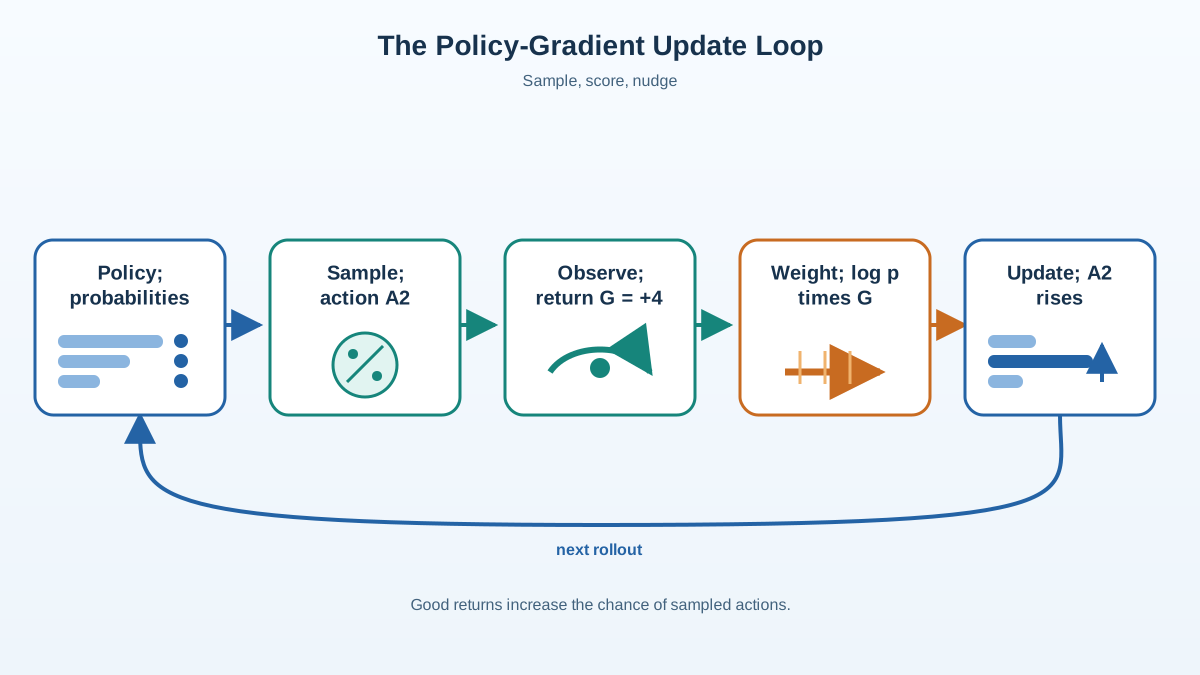
Let's get concrete about the mechanism, because the name "policy gradient" hides how simple the underlying loop actually is.

A parameterized policy maps a state to a probability distribution over actions. Not to a single chosen action—to a distribution. In a two-action environment, the policy might say "take action A with probability 0.7, action B with probability 0.3." Those probabilities are controlled by parameters, and training means adjusting those parameters.

The agent then rolls out a trajectory by sampling actions from the current policy. It doesn't take the most probable action every time. It samples, the way you'd draw a card from a weighted deck. This sampling step is not a minor implementation detail. It's the engine that drives both exploration and learning.

Here's the update rule in plain language:

Actions that led to higher-than-usual return get their probabilities nudged up. Actions that led to lower return get nudged down.

That's the entire intuition. The mechanism that makes it work is the log-probability trick. When the agent takes an action, it records the log-probability of that action under the current policy. After the episode finishes and the return is known, the algorithm multiplies that log-probability by the return and uses the result as a gradient direction.

Let's make this concrete with a tiny numeric example. Suppose your agent faces a two-action choice. Action A returns about +4 on average. Action B returns about -1. The policy starts roughly balanced, 50/50.

The agent samples action A and observes a return of +4. The update computes the gradient direction that would increase action A's probability, then weights that direction by +4. The result: action A's probability creeps up.

Next episode, the agent samples action B and observes -1. The update weights action B's log-probability by a negative return, so action B's probability creeps down.

Notice what's happening: each episode credits the return to every action that was sampled along the way. If the agent took action A, then later took action C, the return from that episode nudges both probabilities—though later actions get weighted more heavily through the discounted return-to-go. One episode is weak evidence about any single action, which is exactly why the updates are small.

After enough episodes, the policy might sit at 90/10 or even 99/1 in favor of action A. The key word in that example is slightly. Each update is a small nudge, not a leap. The policy changes gradually because each individual trajectory is just one sample of what the environment can produce.

Why Stochastic Policies Matter

If you came from Q-learning, the stochastic nature of policy gradient methods might feel like a bug. It's not. It's a feature with real consequences.

Value-based methods typically converge toward deterministic greedy policies. Once the Q-values are confident enough, the agent always takes the same best action. Exploration becomes a separate mechanism—epsilon-greedy, where the agent occasionally takes a random action just to gather information.

Policy gradient methods fold exploration into the policy itself. Because the agent samples actions from a distribution, randomness is structural. The policy doesn't need a separate exploration schedule bolted on. It explores by being stochastic, and it becomes more deterministic only as training pushes probabilities toward confident choices.

This matters for a deeper reason. Some environments genuinely reward stochastic behavior. Consider a simple repeated game where your opponent can observe your strategy. If you always play the same move, they'll counter it. The optimal policy is a mixed strategy—randomize in specific proportions. A standard greedy value-based policy can't represent that. A stochastic policy can.

But the analogy has a boundary. Stochastic policies are not automatically better. As training progresses, the policy tends to sharpen toward exploitation—probabilities drift toward 1 or 0. That's usually what you want, but it can trap the agent in local optima. Once the policy commits to a decent-but-not-optimal region of behavior, the sampling that would discover something better becomes increasingly unlikely. The policy's growing confidence becomes a cage.

Where High Variance Enters the Update

Here's the weakness that defines vanilla policy gradient methods: the gradient estimate is built from a handful of sampled trajectories, and sampled trajectories are noisy.

Think about what one episode actually tells you. The return depends on the actions the policy took, sure. But it also depends on the environment's randomness, the luck of the rollout, and every decision made along the way. Two trajectories from the same policy can produce wildly different returns. One episode where the agent stumbles into a lucky sequence of states might produce a great return. The next episode, same policy, same parameters, might produce a disaster.

The update can't tell the difference between "that action was genuinely good" and "that action happened to be followed by a lucky sequence of events." It just sees the return and pushes the probability accordingly.

REINFORCE, the simplest policy gradient algorithm, is especially prone to this. It uses the full Monte Carlo return from each episode as its signal, and full returns have high variance. The observable symptoms are familiar to anyone who has trained one of these agents:

• Training curves that bounce around instead of climbing smoothly.
• Policies that seem to improve, then regress.
• Results that change dramatically with different random seeds.

The first variance-reduction lever is the baseline. Instead of weighting an action's log-probability by the raw return, subtract a value estimate from the return first.

Here's the causal translation: the baseline is an expected-return reference for the state you were in. The advantage is the sampled return minus that reference. What matters isn't whether an action produced a high absolute return. What matters is whether it did better than expected. If the baseline prediction for a state is +5 and the agent got +6, that action was genuinely good. If the baseline was +5 and the agent got +1, that action was worse than expected—even if +1 isn't negative.

Note that the baseline doesn't need to identify the best alternative action. It's a reference point for comparison, not a competitor. The baseline doesn't change what the policy is learning. It changes the noise around that learning. By centering the update signal around zero—better than expected pushes up, worse than expected pushes down—you remove a huge source of variance that comes from the environment's inherent unpredictability.

From REINFORCE to Actor-Critic Reasoning

Once you understand the baseline, the next step in policy gradient reinforcement learning almost designs itself. If a value estimate helps reduce variance, why not learn one alongside the policy and use it continuously?

That pairing has a name: actor-critic. The actor is the policy, deciding which actions to take. The critic is the value estimate, judging how good the resulting states or actions actually were. The critic gives the actor a more stable reference than raw sampled returns, and the actor uses that reference to decide which direction to push its probabilities.

The reasoning shifts from "how much return did this trajectory produce?" to "did this action do better than the baseline expectation for this state?" That difference—between what happened and what was expected to happen—is the advantage. It's the signal that tells the actor which way to lean.

This is the conceptual bridge from vanilla policy gradients to the modern family of policy optimization methods. Algorithms like PPO build on this foundation, adding mechanisms to keep updates stable and prevent the policy from changing too drastically in one step. But the core insight is the same one you've already absorbed: sample actions, observe outcomes, compare against expectation, and nudge probabilities in the direction of what worked.

One honest caveat before you go build something: vanilla REINFORCE is sample-hungry. It needs many trajectories to average out the noise, and it needs careful tuning of learning rates and other hyperparameters. In a simple discrete environment where Q-learning converges quickly, reaching for a policy gradient method is overkill. Save it for the problems where value-based methods genuinely struggle.

Common Mistakes Beginners Make

Moving from value-based intuition to policy gradients trips up almost everyone in the same few places. Here are the ones I see most often.

Treating the policy as deterministic. If you forget that sampling is what drives exploration, you'll be confused about why the agent sometimes takes suboptimal actions late in training. It's supposed to. That randomness is the mechanism.

Trusting a single trajectory. One great episode or one terrible episode is not evidence. The gradient estimate is noisy by construction. Judge the policy by its behavior over many episodes, not by the last rollout.

Ignoring the on-policy constraint. Vanilla REINFORCE is on-policy: the data used for an update must come from the current policy, not from old experience or a replay buffer. If you update with stale trajectories, you're estimating the gradient for a policy that no longer exists. Reusing old data is possible, but it requires a different objective or an off-policy correction—you can't just feed a replay buffer into the vanilla update.

Expecting monotonic improvement. The loss curve for a policy gradient agent doesn't look like a clean gradient descent curve. It looks like a noisy mountain hike—progress punctuated by setbacks. That's normal.

Reaching for a complex algorithm before understanding the vanilla version. If you can't diagnose why REINFORCE is failing, PPO won't save you. The variance problem doesn't disappear with a more sophisticated algorithm. It gets managed. Understanding the failure mode first is what makes the advanced methods make sense.

The Experiment That Makes It Click

The fastest way to internalize policy gradient reinforcement learning is to watch a policy's probability distribution shift in real time. Pick a simple environment with a small discrete action space. Implement the vanilla REINFORCE loop: sample actions from the current policy, collect a full episode, compute the discounted return, and update the policy parameters using the log-probabilities weighted by those returns.

Then watch what happens. Early episodes, the distribution hovers near uniform—the agent is exploring everything. As training progresses, you'll see probabilities drift. Good actions gain mass. Bad actions lose it. And you'll also see the variance firsthand: episodes where the return spikes or crashes for reasons that have nothing to do with the policy's quality.

That observation—seeing the noise and the signal mixed together in one training run—is worth more than any abstract explanation of variance. It's the foundation you'll need for the next step: what happens when neural networks enter the picture and policy gradient methods scale to problems with high-dimensional observations.

References

Research updated Sep 9, 2026