Proximal Policy Optimization Explained: Why Clipped Updates Can Stabilize Policy Learning

A policy-gradient update is a stride, not a leap. Take too long a step, and you can land somewhere worse than where you started—sometimes so much worse that the policy never recovers. Proximal policy optimization (PPO) is the mechanism that lets the policy take the biggest useful step without stepping off a cliff.

The Problem PPO Solves: When a Big Gradient Step Backfires

Recall how a policy-gradient update works. You collect experience by running your current policy, estimate how much better or worse each action was than expected, then nudge the policy parameters to make good actions more likely and bad actions less likely. The gradient tells you which direction improves the objective, but it does not tell you how far to go.

That missing distance is where training runs die.

The data you collected came from the old policy. If you take an aggressive step, the new policy can drift into regions where those samples no longer represent what the policy would actually do. The gradient estimate was built on actions the old policy tended to take. Once the new policy assigns very different probabilities to those same actions, the estimate becomes stale—and the update that looked good on paper can collapse performance in the environment.

Think of it as walking across uneven terrain in the dark. The gradient tells you the direction of the slope, but it cannot tell you whether the ground ten meters ahead is solid. Take one confident stride, and you might find out the hard way.

This is the trust-region idea: an update is only trustworthy close to where the data was collected. Earlier algorithms like TRPO enforced this with a hard constraint on how far the new policy could move from the old one, measured by KL divergence. It worked, but it required computing second-order information—expensive and complicated to implement.

PPO asks a simpler question: what if we kept the update first-order and simply removed the incentive to drift too far? That is the job of the clipped objective.

The Probability Ratio: Reweighting Stale Data

Before clipping can constrain anything, PPO needs a way to compare the new policy against the one that collected the data. The probability ratio is that comparison.

For each state-action pair in your collected batch, the ratio is:

[ r_t(\theta) = \frac{\pi_\theta(a_t|s_t)}{\pi_{\theta_{\text{old}}}(a_t|s_t)} ]

In plain terms: how much more or less likely does the new policy make an action that the old policy actually took?

Three regimes matter:

• Ratio near 1: The new policy assigns roughly the same probability. Little has changed for this sample.
• Ratio above 1: The action became more likely under the new policy.
• Ratio below 1: The action became less likely.

A concrete example makes this tangible. Suppose the old policy chose "move left" with probability 0.4 in a particular state. After one update, the new policy assigns probability 0.6. The ratio is 1.5. The action is now 50% more likely than before. If the new policy instead assigned 0.2, the ratio is 0.5—the action got cut in half.

Why does this ratio matter? Because it lets PPO reweight old-policy data as if it came from the new policy. This is importance sampling in disguise: instead of recollecting experience after every update, PPO multiplies each sample's contribution by how the probability of that action has shifted. The ratio tells the optimizer how much each piece of old data should count under the new policy.

One qualification matters here, because it is easy to overgeneralize the ratio into something it is not. The ratio is a per-sample measure: it compares likelihoods for the specific actions that appear in your batch. It is not a complete measure of distance between two policies. The new policy could keep every sampled ratio near 1 while changing its behavior dramatically in states the batch never covered. And because PPO typically runs several minibatch epochs over the same collected data, the policy being updated drifts further from the data-generating policy with every pass. The ratio is a useful ruler for what the objective sees—not a certificate that the policies are globally close.

The Clipped Objective: Why a Ceiling and a Floor Keep Updates Honest

The ratio alone does not constrain anything. A vanilla policy-gradient objective would happily multiply the ratio by the advantage and push the policy as far as the gradient suggests. PPO's contribution is to cap how much the objective can benefit from drift.

The clipped surrogate objective looks like this:

[ L(\theta) = \mathbb{E}_t\left[\min\left(r_t(\theta) A_t,; \text{clip}(r_t(\theta), 1-\epsilon, 1+\epsilon) A_t\right)\right] ]

Read it as two competing terms. The first is the unclipped, importance-weighted advantage—the standard policy-gradient objective. The second is the same quantity with the ratio clamped between (1-\epsilon) and (1+\epsilon). Taking the minimum of the two means the objective can never claim more credit than the clipped version allows.

The asymmetry is where the cleverness lives.

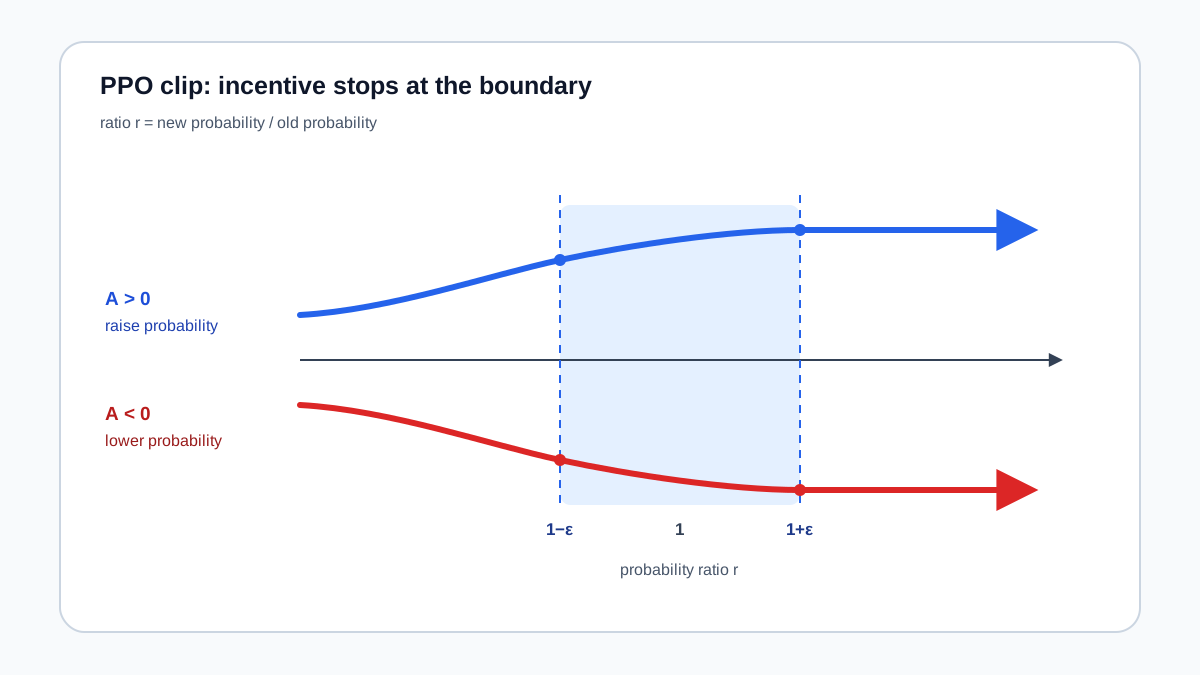
When the advantage is positive—the action was better than expected—the update wants to make that action more likely. The ratio rises above 1. Once it crosses (1+\epsilon), the clipped term stops growing. The policy can still make the action more likely, but the objective no longer rewards it for doing so. The gradient incentive flatlines.

When the advantage is negative, the update wants to make the action less likely. The ratio drops below 1. Once it falls beneath (1-\epsilon), the clipped term stops rewarding further decreases. Again, the policy can keep moving, but the objective stops caring.

This is the subtle distinction that trips up many readers: clipping does not forbid large changes. It removes the gradient incentive to make them. The policy is free to drift as far as the optimizer pushes it, but once the ratio passes the clip boundary, that drift stops contributing to the loss. The optimizer has no reason to keep pushing.

The hyperparameter (\epsilon) is the dial that controls how far the new policy can go from the old while still profiting the objective. Typical values land between 0.1 and 0.3. A smaller (\epsilon) means a tighter leash—the policy must stay closer to its previous self to keep earning gradient signal. A larger (\epsilon) permits more movement per update, at the cost of trusting the stale data further.

If you plotted the clipped objective against the ratio, you would see the curve rise with the ratio, then flatten abruptly at the clip boundary. That flat region is the mechanism doing its work: the gradient is zero there, so the optimizer has nothing to gain by pushing further.

Note: PPO-Clip is inspired by trust-region reasoning, but it is not the same as enforcing a KL-distance constraint. TRPO explicitly bounds how far the new policy can move. PPO clips contributions to the objective and lets the optimizer decide the actual parameter step. The two often behave similarly in practice; they are not the same mechanism.

Why PPO Is an Actor-Critic Method (and What the Critic Actually Does)

PPO sits firmly in the actor-critic family. The actor is the policy network whose probability ratio gets clipped. The critic is the value network that supplies the advantage estimates weighting each update.

The division of labor matters. Clipping constrains the actor's update, but the critic learns normally. The value network keeps regressing toward the observed returns, improving its estimates of how good each state actually is. Those improving estimates feed better advantage signals into the next policy update.

The advantage estimates themselves typically come from generalized advantage estimation (GAE), which balances bias and variance by trading off how many future rewards each estimate includes. Short horizons bias the estimate toward immediate rewards; long horizons add variance from noisy returns. GAE's parameter lets you choose where to sit on that spectrum.

Keep this section short because the architecture itself deserves its own treatment. What matters here is the division of labor: the critic learns what good means, and the clipped actor update decides how far to move toward it.

What PPO Does and Does Not Guarantee

Here is where the "PPO just works" myth needs correcting.

PPO provides no monotonic improvement guarantee. TRPO came with a theoretical bound on how much the policy could degrade between updates. PPO's clipping is a heuristic that approximates a trust region with first-order optimization—cheaper and simpler, but without the formal safety certificate.

What clipping actually buys you is more modest and more practical:

• Reduced variance in updates: The objective cannot reward extreme ratio swings, so individual gradient estimates carry less wild variation.
• Tolerance for larger step sizes: Because the loss flattens beyond the clip boundary, you can use bigger learning rates without the update running away as easily.
• First-order simplicity: No Hessian computation, no conjugate gradient solves. Just standard stochastic gradient ascent.

The failure modes are real. PPO can still collapse if the learning rate is too high, if the advantage estimates are poor, or if the policy overfits the collected batch by taking too many optimization epochs over the same data. The clip boundary protects against one specific failure—gradient incentive to drift—not against every way training can go wrong.

What is known: clipping removes the gradient incentive for the policy to drift far from its previous configuration. What is inferred from practice: this reliably prevents the kind of catastrophic collapse that plagues vanilla policy gradients. What should not be assumed: that PPO is universally stable, sample-efficient, or the right tool for every RL problem.

PPO suits online, on-policy problems with moderate sample budgets. If you have an off-policy setting with a replay buffer, or a problem where sample efficiency dominates every other concern, other algorithms may serve you better. PPO is a workhorse, not a magic recipe.

Reading a PPO Training Run: What to Watch For

The mechanism gives you concrete signals for debugging. Watching the loss curve alone will mislead you—the clipped objective is designed to flatten, so a flat loss can mean healthy convergence or a policy that stopped learning.

Watch the ratio distribution alongside other signals.

In a typical run, most probability ratios stay near 1. The policy drifts gradually, and the clip boundary rarely binds. Reward climbs with bounded variance, and advantage estimates stay within a reasonable range.

Warning signs appear when the ratios cluster at the clip boundary. If most samples sit pinned at (1+\epsilon) or (1-\epsilon), the objective is saturated: the policy is trying to move faster than the clip allows. That can mean your learning rate is too high, your batch is too small to estimate the gradient reliably, or you are running too many epochs over the same data. The policy is straining against the leash on every update—and the leash is the only thing keeping it from collapse.

But resist the urge to turn one metric into a verdict. A high clip fraction is a warning to investigate, not proof of imminent collapse. A low clip fraction does not prove useful learning—the policy could be moving too slowly to improve, or drifting in states your batch never sampled. The honest way to read a PPO run is to triangulate: watch the clip fraction alongside approximate KL divergence, reward trend, entropy, value loss, and the advantage scale. Boundary saturation plus rising value loss and collapsing reward tells a different story than boundary saturation with healthy reward growth.

A reward collapse after an update is the most obvious failure, but subtler problems show up earlier. Watch the value loss diverge from the policy loss, or watch the ratio distribution shift from centered to skewed. Both signal that the actor and critic are falling out of sync.

The practical experiment I would run: take a small continuous-control task, implement PPO with logging for the ratio statistics, and deliberately set (\epsilon) too large and then too small. Watch what happens to the ratio distribution and the reward curve in each case. You will feel the clip boundary change the update behavior in a way that reading equations cannot teach.

PPO is a mechanism that removes the gradient incentive to drift—not a guarantee of stability. Understand the ratio, respect the clip boundary, and treat the training curve as evidence about whether your policy is learning or merely straining against its leash. Run the experiment, log the ratios, and let the output teach you the rest.

References

Research updated Sep 9, 2026