
Deriving the Bayesian Belief Update for a POMDP
The agent never sees the state. It sees a flicker of evidence, acts, and sees another flicker. Yet the entire decision problem collapses into a fixed-size…

Key topics
The agent never sees the state. It sees a flicker of evidence, acts, and sees another flicker. Yet the entire decision problem collapses into a fixed-size vector of probabilities. This article derives that collapse.
You already know what a belief is: a probability distribution over hidden states that stands in for the state you cannot observe. What you probably have not done is build the update rule from scratch. Most treatments hand you the formula and move on. That is a mistake, because the formula is where the interesting reasoning lives — and where most implementation bugs hide.
Let's earn it.
The History Problem and Why a Vector Can Replace It
Start with the real difficulty. At time , the agent's information is a history:
That sequence grows without bound. A policy over histories is a function from an ever-lengthening object to an action, and you cannot tabulate it, store it, or learn it directly. The history is a moving target.
In a fully observable MDP, this problem does not exist. The current state is already a sufficient statistic for the future: given , nothing older changes the distribution over what happens next. That is the Markov property, and it is what makes MDPs tractable.
A POMDP loses that property at the level of what the agent observes. The observation alone is not sufficient — it is a noisy, partial glimpse. But the underlying process is still Markov in the true state. The past matters only through the current state distribution. That single fact is the crack of light we are going to widen into a full derivation.
The claim we have to earn: the belief — a probability vector over states — is a sufficient statistic for . Conditioning on loses nothing for decision-making. If that is true, the unbounded history collapses into a fixed-size vector, and the POMDP becomes a decision problem over beliefs.
Notation: States, Actions, Observations, and the Two Models
Before the derivation, name every symbol and tie it to a mechanism.
- : finite set of hidden states.
- : finite set of actions.
- : finite set of observations.
- : a probability vector over , where is the agent's current belief that the true state is .
Two models drive everything:
- Transition model : the probability the world moves to after taking action in state . This is where the world goes, independent of what the agent sees.
- Observation model : the probability of perceiving observation after taking action and landing in state .
Read the second one carefully. The observation depends on the resulting state , not the previous state . Almost every derivation error I have seen comes from getting this order wrong. The world moves first; the sensor fires second.
The belief lives on a simplex: every entry is non-negative and the entries sum to one. That constraint is not decoration. It is what forces normalization to be a required step rather than a cosmetic cleanup.
Step 1 — Predict: Propagating Belief Through the Transition Model
Suppose the agent holds belief and takes action . Before any new observation arrives, where does the belief go?
The world could reach from any previous state . Sum over all of them, weighted by how likely each starting state was:
Read it as: every way the world could have reached , weighted by how much belief we had in each starting point. This is marginalization — you are summing out the unknown previous state.
Notice what this step does to the belief. Transitions redistribute probability mass according to where the dynamics send it. If the transition model tends to spread mass across states, the predicted belief gets flatter. If it funnels mass toward a few states, the predicted belief can get sharper than the prior. Prediction is not a blur. It is a weighted reallocation, and the direction depends entirely on the transition structure.
In matrix form, if you stack as a column vector and let be the matrix with entries , the prediction is a vector-matrix product:
It is a linear operation. That linearity is worth remembering — it is why belief updates are cheap to compute even when planning over beliefs is not.
One more thing: this step is exactly where a model-free agent has nothing to work with. The prediction requires . That is why this derivation assumes known dynamics, and why model-free POMDP methods have to learn or bypass this step entirely.
Knowledge check
Check your understanding
Answer this question before you continue.
Step 2 — Correct: Weighting by the Observation Likelihood
Now an observation arrives. Apply Bayes' rule to the predicted belief. The posterior is proportional to the likelihood times the prior:
The tilde marks this as unnormalized. We will fix that in the next step.
The mechanism in plain terms: states that make the observed signal likely gain mass; states that make it unlikely lose mass. If you observe a reading that is nearly impossible under state , that state's probability collapses toward zero.
That collapse is permanent for this posterior. A state driven to exactly zero by an impossible observation stays at zero until the next prediction step. Then the transition model gets its turn again: if other states can transition into , probability mass flows back in. The zero is not a death sentence — it is a temporary verdict that the next prediction can overturn. The exception is a state with no incoming transitions from any state with positive belief, which is genuinely unreachable and stays dead.
Contrast the two steps. Prediction reallocates uncertainty according to the dynamics. Correction concentrates it around whatever the evidence supports. They pull in different directions, and the recursion is the tension between them.
Knowledge check
Check your understanding
Answer this question before you continue.
Step 3 — Normalize: Why the Denominator Is Not Optional
The unnormalized posterior does not sum to one. To restore a valid probability distribution, divide by the total mass:
The denominator is the probability of observing given the belief and action. It is the model's own prediction of the evidence you just received.
That interpretation is not just poetry — it is a diagnostic. Watch that number in your code. A persistently tiny denominator means the model does not expect what the environment keeps producing. That is a signal worth investigating: check your observation likelihoods, check whether the sensor model matches reality, check whether the environment has drifted. A small denominator alone does not prove a bug — rare but valid observations also produce low likelihoods. But when the number keeps dropping, the model and the world are disagreeing about what is plausible. Normalization is where the model confesses.
Putting all three steps together, the full recursion is:
This is the POMDP belief update equation. It is equivalent to the standard Bayes filter, and in the hidden Markov model literature it is the forward algorithm. Same recursion, different name.
Knowledge check
Check your understanding
Answer this question before you continue.
Worked Example: One Predict-Update-Normalize Cycle by Hand
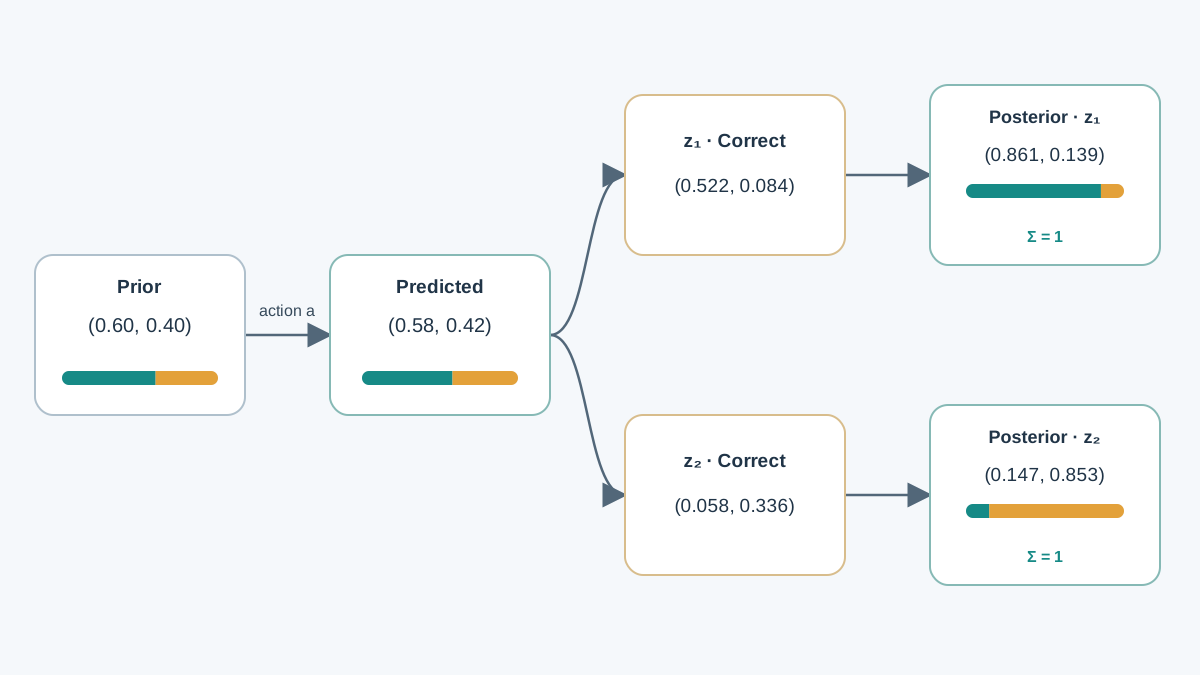
Two states, two actions, two observations. Small enough to check by hand.
States: . Actions: . Observations: .
Prior belief: , .
Transition model for action :
| 0.7 | 0.3 | |
| 0.4 | 0.6 |
Observation model for action :
| 0.9 | 0.1 | |
| 0.2 | 0.8 |
Predict. Take action :
The prior was ; the prediction is . Slightly flatter here, because this particular transition matrix spreads mass. Change the transition probabilities and you can get a sharper prediction instead.
Correct. Suppose you observe :
Normalize. The total mass is :
Check: . Good.
Now branch from the same prediction and observe instead:
Total mass :
Same prior, same action, two observations, two opposite posteriors. That is the whole point of the correction step: evidence reshapes belief.
Read the result as a decision input. After observing , the agent is fairly confident it is in ; after , it is fairly confident it is in . Which action looks better now depends on the reward structure and on how the belief will evolve — that is POMDP planning, and it belongs to the value machinery, not to this derivation.
Knowledge check
Check your understanding
Answer this question before you continue.
Why the Belief Is Sufficient — and When It Is Not
Look back at the recursion. The right-hand side uses only , , and . Nothing older appears. That is not a coincidence; it is the proof. If the update from to depends on nothing before , then carries all the information the history carried for the purpose of predicting the future. The belief is a sufficient statistic for the history.
This is what lets you view the POMDP as a belief MDP: a Markov decision process whose states are beliefs. The state space is continuous — even for a finite POMDP, the set of distributions over states is infinite — but the Markov property holds, so Bellman-style reasoning still applies. That is the bridge to value functions over beliefs.
The result rests on assumptions. Name them:
- The transition and observation models are known and correct.
- The true process is Markov in the state.
- The belief is actually maintained, not approximated away.
Break any of these and the vector stops being sufficient. A misspecified observation model makes the correction step lie. A state space that omits a relevant hidden variable makes the Markov assumption false. A compressed belief that drops information — a low-dimensional summary, a discretization, a learned encoder — is no longer the sufficient statistic, and the agent's decisions degrade quietly rather than loudly.
There is also a practical cost. Maintaining the belief is cheap: it is a sum and a product per state. Planning over beliefs is not. The belief space is continuous, and exact optimal policies over it are generally intractable. Cheap to track, expensive to optimize — that asymmetry is the central engineering fact of POMDPs.
Common Derivation Mistakes to Check Against
When your belief update misbehaves, run this checklist against the derivation itself:
- Indexing the observation model by the previous state. It is , not . The world moves first.
- Forgetting to normalize, or normalizing before the correction instead of after. The denominator belongs at the end.
- Skipping the prediction step and correcting directly from the old belief. That silently drops the effect of the action.
- Assuming a zeroed state stays zero forever. It stays zero for the current posterior, but the next prediction can restore mass if other states transition into it. Only a state with no incoming transitions from reachable states is permanently dead.
- Confusing the belief update with a value update. This recursion tracks what the agent knows, not how good anything is. Mixing them is a category error.
Common mistake: treating the denominator as a formality. It is the model's predicted probability of the observation you just received. Log it. A number that keeps dropping toward zero is telling you the model and the environment disagree about what is plausible — inspect the observation likelihoods before assuming the math is wrong.
Where This Leaves You
The belief is a running summary. Prediction reallocates probability according to the dynamics. Correction concentrates it around the evidence. The recursion is the entire mechanism, and it fits in one line.
Here is the next move I would make. Implement the three steps for the two-state example above. Print the belief after each step. Watch the sum stay at one. Then run two experiments. First, feed it an observation that is impossible under one state and watch that state's probability drop to zero — then take another prediction step and watch whether mass flows back in. If your transition model allows other states to reach it, the state recovers. If not, it stays dead. Second, change the transition matrix so that mass funnels toward a single state and watch the prediction get sharper instead of flatter. Those two experiments will teach you more about belief filtering than any amount of staring at the formula.
Once you trust the recursion, the belief becomes the state over which value and policy reasoning happens. That is the belief MDP, and it is where the next layer of the POMDP story begins.
Knowledge check
Final check
Finish the article by checking the ideas you just learned.
References
Build a stronger RL mental model
Use structured resources to connect equations, algorithms, and observable agent behavior.


