Practice POMDP Belief Updates With a Small Python Example

You can recite the belief update formula and still have no idea whether you are applying it correctly. The way out is not more reading. It is a two-state problem small enough that every number is checkable by eye.

This is a drill. We will build the smallest useful partially observable Markov decision process (POMDP), run a belief update step by step, print every intermediate value, and then use the resulting belief to compare two actions. If you already accept that a belief is a probability distribution over hidden states and a sufficient summary of history, you have everything you need. If that sentence felt shaky, spend ten minutes with the belief-state mental model first, then come back. Here we only compute.

What We Are Building and What You Need

The running problem: a hidden light that is either on or off. You cannot see it directly. You can take one of two actions:

• wait — the light tends to stay where it is.
• toggle — the light tends to flip.

After each action you receive a noisy observation: bright or dark. The sensor is right most of the time, not always.

Two states is the right size for a first drill because the belief is a single number. If p is the probability the light is on, then 1 - p is the probability it is off. Every step is verifiable with mental arithmetic.

Dependencies: Python 3 and NumPy. No RL library, no credentials, no external services.

We need four tables:

Table	Meaning
T[action][s, s']	Probability of landing in s' given you were in s and took action
O[action][s', o]	Probability of seeing o given you landed in s' after action
b0	Initial belief over states
R[action][s]	Immediate reward for taking action in s

The expected output for the whole exercise: a printed belief vector after each action-observation step, plus a normalization check that sums to 1.0.

The Two-Step Update, Separated

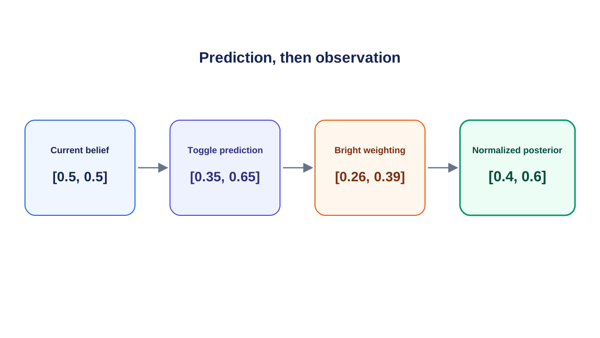
The belief update is two operations wearing one formula. Split them and the confusion mostly disappears.

Prediction (the action step). Push the current belief through the transition model. This gives a prior over next states — where you probably are after your action, before you see anything.

Correction (the observation step). Multiply that prior by the likelihood of the observation under each candidate next state, then normalize.

The order matters. The action changes where you probably are. The observation changes what you believe about where you are. Skip the prediction step and your belief reacts to observations while ignoring the effect of your own choices — the single most common bug in hand-rolled belief updates.

The normalizer is not decoration. It is the total probability of the observation you actually saw, and it doubles as a surprise meter: a small normalizer means the observation was unlikely under your prior.

Step 1: Predict the Belief After an Action

Prediction is a matrix-vector product. For action a, build the transition matrix T_a where row s holds the distribution over next states. To compute the prior over next states, we need to weight each row by the current belief and sum:

b_prior[s'] = Σ_s b[s] * T_a[s, s']

In matrix form, that is b_prior = b @ T_a, or equivalently T_a.T @ b if you prefer column vectors. We will use b @ T_a to keep the row convention explicit.

import numpy as np

STATES = ["off", "on"]
ACTIONS = ["wait", "toggle"]
OBS = ["dark", "bright"]

# T[action][s, s'] : rows sum to 1
T = {
    "wait":   np.array([[0.9, 0.1],
                        [0.2, 0.8]]),
    "toggle": np.array([[0.2, 0.8],
                        [0.7, 0.3]]),
}

def predict(b, action):
    return b @ T[action]

b0 = np.array([0.5, 0.5])
b_prior = predict(b0, "toggle")
print("prior:", b_prior, "sum:", b_prior.sum())

Expected output:

prior: [0.35 0.65] sum: 1.0

Two sanity checks worth running before you trust anything downstream:

• Deterministic action. If toggle always moved off to on, then [1.0, 0.0] must become [0.0, 1.0].
• No-op action. An identity transition must leave the belief unchanged. This is the fastest way to catch a transposed matrix.

Common mistake: building T as columns instead of rows. The prior still sums to 1.0, so nothing screams at you — it is just quietly wrong. The no-op check catches it in one line.

Step 2: Update With an Observation

Now correct the prior with what you actually saw. Multiply elementwise by the observation likelihood column for the received observation, then normalize.

# O[action][s', o]
O = {
    "wait":   np.array([[0.7, 0.3],
                        [0.3, 0.7]]),
    "toggle": np.array([[0.6, 0.4],
                        [0.4, 0.6]]),
}

def correct(b_prior, action, obs):
    o_idx = OBS.index(obs)
    b_unnorm = O[action][:, o_idx] * b_prior
    normalizer = b_unnorm.sum()
    return b_unnorm / normalizer, normalizer, b_unnorm

b_post, z, b_unnorm = correct(b_prior, "toggle", "bright")
print("unnormalized:", b_unnorm)
print("normalizer:  ", z)
print("posterior:   ", b_post, "sum:", b_post.sum())

Expected output:

unnormalized: [0.26 0.39]
normalizer:   0.65
posterior:    [0.4 0.6] sum: 1.0

Read the normalizer as a statement about surprise. Here it is 0.65 — seeing bright after toggle was reasonably likely under your prior. If it had come out at 0.05, either your model is off or your belief was.

Common mistake: forgetting to normalize and feeding the unnormalized vector into the next step. The belief drifts, and eventually you get probabilities above 1.

Run It: A Full Two-Step Trace

Now loop the whole pipeline: choose an action, predict, receive an observation, correct, print. Fix the seed so your trace is reproducible.

rng = np.random.default_rng(7)

def sample_observation(b_prior, action):
    probs = b_prior @ O[action]   # P(o | b_prior, action)
    return rng.choice(OBS, p=probs)

b = b0.copy()
for step in range(1, 4):
    action = "toggle" if step % 2 else "wait"
    b_prior = predict(b, action)
    obs = sample_observation(b_prior, action)
    b, z, _ = correct(b_prior, action, obs)
    print(f"step {step} | a={action:6s} | o={obs:6s} | "
          f"b={np.round(b, 3)} | sum={b.sum():.3f} | z={z:.3f}")

A representative trace:

step 1 | a=toggle | o=bright | b=[0.4 0.6] | sum=1.000 | z=0.650
step 2 | a=wait   | o=bright | b=[0.316 0.684] | sum=1.000 | z=0.574
step 3 | a=toggle | o=dark   | b=[0.591 0.409] | sum=1.000 | z=0.554

What to look for: beliefs that sharpen toward one state when observations are informative, and beliefs that hover near 0.5 when they are not. The sum column is your proof that the arithmetic is intact.

Compare Two Candidate Decisions From the Belief

The belief is not a souvenir. It is the thing you decide from. Score each action by expected immediate reward, weighted by the belief:

R = {
    "wait":   np.array([0.0, 1.0]),   # reward per state
    "toggle": np.array([0.5, 0.5]),
}

def expected_reward(b, action):
    return float(b @ R[action])

b = np.array([0.4, 0.6])
for a in ACTIONS:
    print(a, round(expected_reward(b, a), 3))

With b = [0.4, 0.6], wait scores 0.6 and toggle scores 0.5. The belief says wait wins.

This reward table is a separate toy decision layer, not a consequence of the light-state transition model above. Its job is to show the mechanics: once you have a belief, you can score actions by weighting each state's reward by the probability you are in that state. The belief from the previous section — [0.4, 0.6] — is exactly the posterior we computed, so the decision follows directly from the update.

Now suppose your last observation was bright. A policy that acts on the raw observation might pick toggle — bright suggests the light is on, and toggling feels productive. The belief says otherwise, because it has already folded in the action you took and the sensor's noise. The belief wins because it is a sufficient statistic; the last observation is not.

Keep this to one-step expected reward. Planning over belief space is a different article.

Tip: if two actions score nearly equal under the current belief, that tie is a signal. An information-gathering action may be worth more than either immediate-reward option.

Break It on Purpose: Three Failure Modes

Deliberate bugs teach faster than correct output. Introduce each one and watch the symptom.

Bug	Symptom	Fix
Skip prediction, update from old belief	Belief reacts to observations but ignores your action	Always run predict before correct
Wrong observation column, or index by state instead of next state	Beliefs move the wrong way after a clear observation	Check O[action][:, o_idx] indexes next states
Drop normalization	Belief sum drifts from 1.0; values stop being probabilities	Divide by b_unnorm.sum() every step

A wrong belief trace tells you exactly which table is wrong. That is more useful than a correct trace you cannot explain.

Your Turn: One Modification Worth Making

Change the observation noise. Make the sensor almost uninformative — set both likelihoods near 0.5 — and run the trace. The belief will barely move no matter what you observe.

Then make it almost perfect — likelihoods near 0.95 — and watch the belief snap to the observed state within one step.

Predict the result before you run it, then compare. The gap between your prediction and the output is the actual lesson: a belief update is a tug-of-war between what you already believed and what you just saw, and the observation model sets the exchange rate.

Optional second variation: start from a skewed initial belief like [0.9, 0.1] and confirm that a few informative observations wash out the initial guess.

Where This Leaves You

A belief update is two separable operations — prediction, then correction — and both are checkable with a sum and a print statement. When a trace looks wrong, check in this order: transition matrix orientation first, observation indexing second, normalization third.

The natural next step is to stop deciding one step at a time and start planning over beliefs, where the value of an action includes the information it buys you. That is where POMDPs get genuinely interesting — and where the arithmetic you just practiced becomes the foundation rather than the exercise.