Why Potential-Based Reward Shaping Preserves Policy Rankings

A shaped agent learns faster, the curve looks great, and the final policy is subtly wrong. The shaping term did not speed up learning; it quietly rewrote the objective.

That failure is common enough that "potential-based reward shaping preserves the optimal policy" gets repeated like a safety certificate. It is a real theorem with a real proof, but the proof leans on specific assumptions, and the slogan hides them. This article derives the result, isolates the boundary term that makes it work, and shows the ways the guarantee breaks.

I assume you already know discounted returns, MDP notation, and the sparse-versus-shaped tradeoff. If not, start with the reward shaping comparison first; here we go straight to the mechanism.

The Claim, and Why It Sounds Too Good

The result, due to Ng, Harada, and Russell, is precise: if you add a shaping reward of the form

$F(s, s') = \gamma \Phi(s') - \Phi(s)$

to a base reward $R$, where $\Phi: S \to \mathbb{R}$ is a bounded potential function and $\gamma$ is the same discount factor used in the return, then the set of optimal policies is unchanged. The optimal value function shifts by a constant offset, but the ranking of policies does not.

The common misconception is weaker and wrong: that any "helpful" or "small" shaping reward is safe. It is not. Arbitrary shaping can reorder policies, and a small shaping term can still flip which policy wins if the base rewards are close together. The guarantee is not about magnitude. It is about structure.

Why bother with the theorem at all? Because it lets you densify a sparse signal without silently rewriting the objective. You get a richer learning signal and keep the same success condition. That trade is worth having, but only if you know what you traded away to get it.

Notation and the Two Reward Functions

Fix an MDP $(S, A, P, R, \gamma)$. For an episodic task, trajectories terminate at a terminal state; for a continuing task, they run indefinitely with discounting. The distinction matters later, so keep it in view.

The base reward is $R(s, a, s')$. The shaped reward is

$R'(s, a, s') = R(s, a, s') + F(s, s').$

The potential $\Phi$ maps states to real numbers and must be bounded. The discount factor inside $F$ must match the $\gamma$ used in the return. That last requirement is not cosmetic; it is the arithmetic that makes the cancellation work.

Define the two returns as expectations over trajectories generated by a policy $\pi$:

$G(\pi) = \mathbb{E}_\pi\left[\sum_{t=0}^{\infty} \gamma^t R(s_t, a_t, s_{t+1})\right], \quad G'(\pi) = \mathbb{E}_\pi\left[\sum_{t=0}^{\infty} \gamma^t R'(s_t, a_t, s_{t+1})\right].$

"Policy ranking is preserved" now has a precise meaning: for any two policies $\pi_1, \pi_2$,

$G'(\pi_1) \geq G'(\pi_2) \iff G(\pi_1) \geq G(\pi_2).$

Everything below is an argument about that equivalence.

The Telescoping Derivation

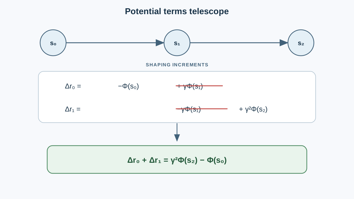
Write the discounted sum of shaping terms along a finite trajectory of length $T$:

$\sum_{t=0}^{T-1} \gamma^t F(s_t, s_{t+1}) = \sum_{t=0}^{T-1} \gamma^t \left[\gamma \Phi(s_{t+1}) - \Phi(s_t)\right].$

Expand the sum term by term:

$= \gamma\Phi(s_1) - \Phi(s_0) + \gamma^2\Phi(s_2) - \gamma\Phi(s_1) + \gamma^3\Phi(s_3) - \gamma^2\Phi(s_2) + \cdots + \gamma^T \Phi(s_T) - \gamma^{T-1}\Phi(s_{T-1}).$

Look at what happens to any interior state $s_t$ with $0 < t < T$. It appears once as $\gamma^t \Phi(s_t)$ from the positive term of step $t-1$, and once as $-\gamma^t \Phi(s_t)$ from the negative term of step $t$. The two cancel exactly. Every interior potential vanishes.

What survives is the first and last term:

$\sum_{t=0}^{T-1} \gamma^t F(s_t, s_{t+1}) = \gamma^T \Phi(s_T) - \Phi(s_0).$

That is the whole mechanism. The shaping term telescopes, and the extra return depends only on where the trajectory starts and where it ends, not on the actions taken in between.

A small numeric check makes the cancellation visible. Take three states with $\Phi(s_0) = 1$, $\Phi(s_1) = 3$, $\Phi(s_2) = 0$, and $\gamma = 0.9$. A trajectory $s_0 \to s_1 \to s_2$ has shaping rewards:

• $F(s_0, s_1) = 0.9 \cdot 3 - 1 = 1.7$
• $F(s_1, s_2) = 0.9 \cdot 0 - 3 = -3.0$

Discounted sum: $1.7 + 0.9 \cdot (-3.0) = 1.7 - 2.7 = -1.0$.

The boundary formula gives $\gamma^2 \Phi(s_2) - \Phi(s_0) = 0.81 \cdot 0 - 1 = -1.0$. Same number. The interior potential of $s_1$ left no trace.

From Boundary Term to Policy Ranking

Now apply the identity to the return. For a fixed start state $s_0$, the term $-\Phi(s_0)$ is a constant across every policy being compared. It shifts all returns by the same amount and cannot change the ranking.

The load-bearing part is $\gamma^T \Phi(s_T)$. For the ranking to be preserved, this boundary contribution must be policy-independent. Two conditions deliver that:

• Zero terminal potential. If $\Phi(s_T) = 0$ on every terminal or absorbing state, the term vanishes regardless of when the episode ends. This is the cleanest sufficient condition.
• Equal terminal potential under a fixed horizon. If every episode runs exactly $T$ steps, $\gamma^T$ is the same constant for every policy, but that alone is not enough: $\Phi(s_T)$ must also be equal across the terminal states that different policies can reach. If all policies terminate in the same state, or if every reachable terminal state shares the same potential value, the boundary term shifts all returns by the same amount.

Either condition is sufficient. Neither is automatic. The invariance condition, stated cleanly: policy ordering is preserved when the boundary contribution is the same for every policy being compared.

The value function shifts accordingly. For a policy $\pi$,

$V'(\pi) = V(\pi) - \Phi(s_0) + \text{terminal correction}.$

The optimal policy is unchanged, but the numbers are not. If you compare two runs by raw shaped return, you are comparing the shaping term, not the task.

Note: The offset is why a shaped agent can report a higher return while behaving identically. The policy is the same; the accounting changed.

Where the Guarantee Breaks

The theorem is only as strong as its assumptions. Audit your shaping function against these failure modes before trusting it.

Arbitrary shaping. If $F$ is not a potential difference, it has no telescoping structure. Each step's shaping reward accumulates independently, so the extra return depends on the actions taken, and policies can reorder. This is the failure the theorem exists to prevent, and it is the one people reintroduce by hand-tuning rewards without checking the form.

Terminal mismatch. If $\Phi$ is nonzero on absorbing states and episodes end at different times under different policies, the surviving $\gamma^T \Phi(s_T)$ term differs across policies. The ranking can flip. The fix is to set $\Phi = 0$ on terminal states, or to ensure the terminal potential is equal across all reachable terminal states under a fixed horizon.

Discount mismatch. Using a different $\gamma$ inside $F$ than in the return breaks the cancellation arithmetic. The interior terms no longer cancel; the proof collapses. This is easy to do accidentally when the shaping function is written in a different module from the return computation.

Time-varying potentials. The static proof assumes $\Phi$ does not change during learning. If you learn or adapt $\Phi$ online, the guarantee needs the difference taken at the times the states were actually visited: $F(s, t, s', t') = \gamma \Phi(s', t') - \Phi(s, t)$. Otherwise the potentials you subtract were never the ones in force when the reward was issued.

A practical audit rule: write your shaping as $\gamma \Phi(s') - \Phi(s)$, confirm $\Phi$ is zero at termination or that all reachable terminal states share the same potential under a fixed horizon, and confirm $\gamma$ matches the return. If any of those three checks fails, the guarantee does not apply, and you are running an experiment with an unknown objective.

What This Buys You in an Experiment

The theorem constrains the objective, not the learning speed. Sample-efficiency gains from shaping are empirical and depend on initialization, potential scale, and the structure of the base reward. A well-chosen potential can help a lot; a badly scaled one can hurt. The theorem says nothing about which.

Because the optimal policy is preserved, a shaped run and an unshaped run are comparable on final policy quality. They are not comparable on raw return magnitude, because the shaped return includes the boundary offset. Evaluate both by the base reward.

That evaluation rule is not optional. If you rank runs by shaped return, you are ranking them by the shaping term, and the run with the most aggressive potential will look best regardless of how well it solves the task.

Keep the potential bounded and log it. When a shaped run produces a suspicious policy, you want to trace the result back to the shaping signal rather than blame the algorithm. A logged potential is the difference between a diagnosis and a guess.

The Decision Rule

Before trusting any shaping term, run it through four checks. Write it as $\gamma \Phi(s') - \Phi(s)$. Confirm $\Phi$ is zero at termination, or that all reachable terminal states share the same potential under a fixed horizon. Confirm $\gamma$ matches the return. Evaluate on the base reward, never the shaped reward.

If all four hold, the policy ranking is preserved and you can use the shaping signal to densify a sparse reward without rewriting the objective. If any fails, you have an arbitrary reward function wearing the costume of a safe one.

The next step is to run the comparison yourself: take a small task, implement the base reward, a potential-based shaping signal, and a deliberately unsafe arbitrary shaping signal, and watch which one preserves the final policy. The derivation tells you what should happen. The experiment tells you whether your implementation actually does it.