
Average-Reward Reinforcement Learning: Learning in Continuing Tasks
Your agent has no finish line. No terminal state ends the run, no episode boundary resets the world, and no natural horizon cuts the future off. You reach…

Key topics
Your agent has no finish line. No terminal state ends the run, no episode boundary resets the world, and no natural horizon cuts the future off. You reach for a discount factor anyway, because that is what the tutorials did—and the agent quietly starts optimizing the wrong thing.
The real question is not which objective looks more elegant. It is what "good" means when the run never ends.
Why Discounted Return Stops Being the Right Question
Discounted return rests on two legitimate foundations. Either the task has a genuine terminal goal that makes the discounted sum a finite-horizon measure, or the discount factor encodes a real time preference: reward now is worth more than reward later because the future is uncertain, capital has opportunity cost, or the run may terminate at any step with fixed probability.
Remove both foundations and the discount factor becomes an arbitrary knob. It still shapes what the agent optimizes, but nothing in the environment justifies the shape it imposes.
The symptom shows up in behavior. Because discounting makes future reward exponentially less important, the agent will sacrifice long-run throughput for a slightly earlier payoff. A server that drains its queue a few steps sooner but leaves the system in a worse steady state looks better to a discounted objective. The agent is not wrong about the math. It is wrong about the question.
The organizing criterion for everything that follows: does success depend on termination, on time preference, or on long-run steady-state performance? Only the third answer points to average reward.
Knowledge check
Check your understanding
Answer this question before you continue.
The Average-Reward Objective: Gain as the Real Target
Average reward reinforcement learning replaces the discounted sum with a rate. For a stationary policy, the gain is the long-run average reward per time step:
[ \rho^\pi = \lim_{T \to \infty} \frac{1}{T} \mathbb{E}\pi \left[ \sum{t=0}^{T-1} r(s_t, a_t) \right] ]
Every time step counts equally. The first step and the millionth step carry the same weight. There is no exponential decay pushing the agent toward short-term gains, because the objective is not a sum at all. It is a rate, and normalizing by the horizon length keeps the quantity finite where an undiscounted infinite sum would diverge.
This is the natural measure for continuing tasks: a queue, a server, a network, a robot that works a shift that never formally ends. Steady-state throughput is the operational goal, and gain is its formal expression.
One structural caveat matters. Under common assumptions—typically that the MDP is communicating or unichain—gain is independent of the starting state. If the MDP can split into recurrent classes the policy never leaves, the long-run rate may depend on where the agent starts. The fix is not to abandon the framing but to specify the objective precisely: evaluate gain from a defined start distribution or a particular recurrent class.
Knowledge check
Check your understanding
Answer this question before you continue.
Bias: The Missing Second Quantity
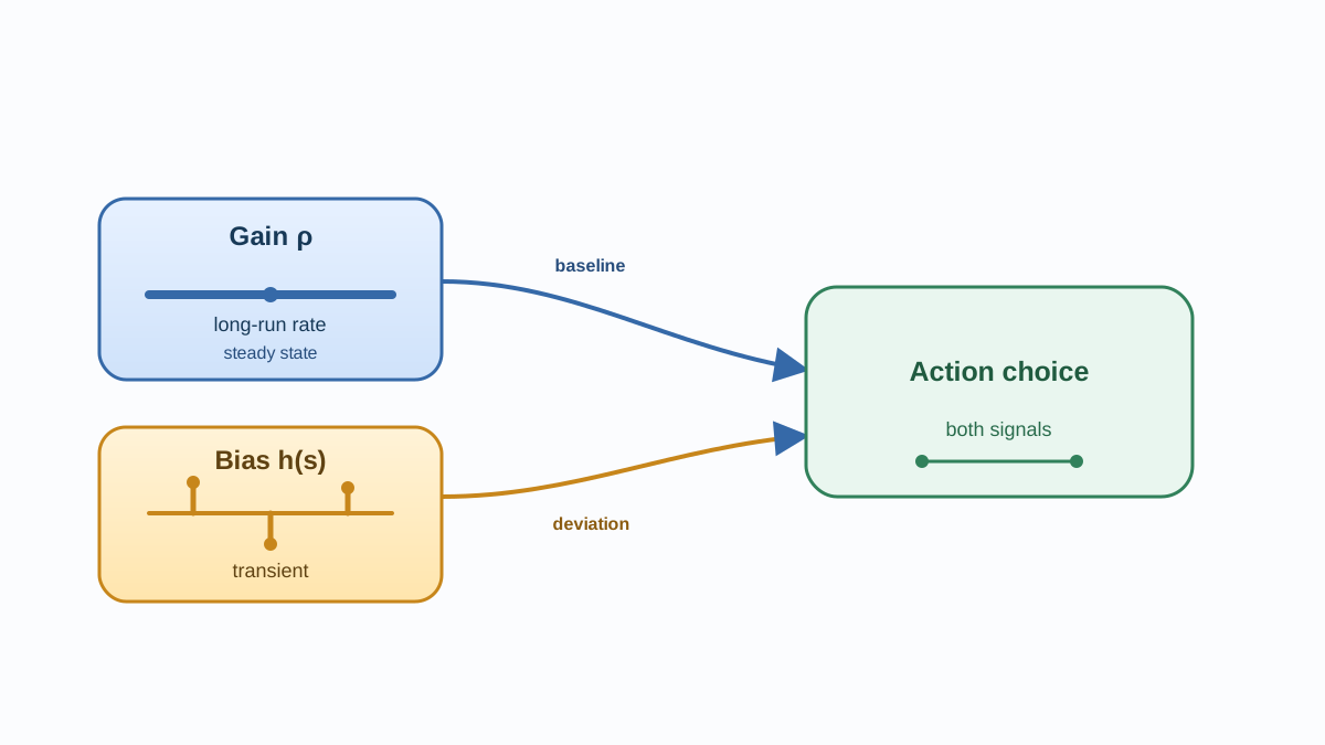
Gain alone cannot drive decisions. It tells you the long-run rate, but not which state you are in or which action is better right now. Two states can share the same gain while one offers a temporary advantage and the other a permanent handicap. The agent needs a second quantity to tell them apart.
That quantity is bias. Bias measures the expected transient advantage of starting in a given state relative to the steady-state average. Think of gain as the river's current and bias as the eddies near the bank. The current tells you where the water is going. The eddies tell you where you are.
The mechanism matters more than the metaphor. In the average-reward Bellman relationship, the immediate reward is adjusted by subtracting the gain, and the continuation term uses bias rather than discounted future value:
[ h^\pi(s) = r(s, a) - \rho^\pi + \mathbb{E}_{s' \sim P(\cdot|s,a)}[h^\pi(s')] ]
The gain anchors the baseline; the bias captures how much better or worse than that baseline this state is right now. Action selection compares these relative signals, which is why the bias function is often described as the analogue of the Q-function in the discounted case. The boundary matters: bias is a relative quantity. It does not predict absolute future reward. It predicts deviation from the steady-state rate before the system settles into its long-run rhythm.
Knowledge check
Check your understanding
Answer this question before you continue.
Average-Reward vs Discounted: A Decision Table
| Discounted Return | Average Reward | |
|---|---|---|
| What it optimizes | Sum of rewards, exponentially weighted by time | Long-run reward rate per step |
| Well-motivated when | Genuine terminal goal, or real time preference | Task runs indefinitely; steady-state rate is the goal |
| No termination | Discount factor becomes an arbitrary modeling choice | Natural fit; no horizon needed |
| Discount factor | Central parameter; reshapes what the agent optimizes | Absent; all steps weighted equally |
| Value-function role | V and Q predict discounted future return | Bias predicts transient advantage over gain |
Deep RL practice blurs this line more than the formalism suggests. Many algorithms train with a discount factor for value estimation while reporting undiscounted or average performance. That hybrid can work, but it inherits a cost: discounted methods with the discount factor close to 1 can approximate average-reward behavior, yet the error bounds scale poorly with the effective horizon. Push the discount factor toward 1 and the approximation improves in principle while the estimation difficulty grows in practice.
Knowledge check
Check your understanding
Answer this question before you continue.
When Average-Reward RL Is the Wrong Tool
Average reward is not a universal upgrade. It is a specific objective for a specific class of problems.
It is a poor fit when the task genuinely has a finite horizon or a meaningful terminal goal. If the agent's run ends, the transient matters, and a rate that ignores the transient throws away information. Average reward also ignores startup costs and one-time windfalls by construction. A short run dominated by its opening phase is not well described by its asymptotic rate.
Practical cost is real. Average-reward algorithms are less mature and less widely supported in tooling than discounted methods. You will write more of the machinery yourself, and you will have fewer battle-tested implementations to lean on. That is a legitimate engineering consideration, not a mark of theoretical weakness.
Choosing Your Objective: A Practical Decision Rule
Ask three diagnostic questions, in order.
Is termination intrinsic to success? If the task ends because reaching the goal is the objective—a maze solved, a delivery completed—you have a finite-horizon or episodic problem. Use discounted return, or no discount at all over the finite horizon.
But be careful: a reset is not the same as a goal. Many continuing systems are split into episodes purely for data collection, while the real operational objective is sustained performance. If the episode boundary is an artifact of training rather than a property of success, do not let it dictate your objective.
Does the future genuinely matter less than the present? If reward now is worth more than reward later because of uncertainty, interest, or termination risk, the discount factor encodes something real. Use it.
Is the goal a steady-state rate? If the system runs indefinitely and success means sustained throughput, average reward reinforcement learning is the objective that matches your problem.
One evaluation habit will save you regardless of which objective you choose: report the metric that matches your deployment objective. If steady-state throughput is the operational goal, report average reward per step even when you train with discounting. The discounted objective shapes learning, but the average rate is what you can compare across runs, across algorithms, and against the true operational goal. If the task is startup-sensitive or genuinely finite-horizon, average reward per step is the wrong report card—use the metric that captures the transient you care about.
The choice cascades. It determines which value function you estimate, which Bellman relationship you write down, which algorithms are available, and how you evaluate the final policy. Naming whether termination is intrinsic, whether time preference is real, and whether steady-state rate is the goal settles the objective first. The rest of the design follows from that decision.
Knowledge check
Final check
Finish the article by checking the ideas you just learned.
References
Research updated Sep 9, 2026


