
The Bellman Equation Explained Through a Decision Tree
The first time you see the Bellman equation, it looks like a symbol puzzle. Greek letters, nested expectations, a value function that seems to appear on…

Key topics
The first time you see the Bellman equation, it looks like a symbol puzzle. Greek letters, nested expectations, a value function that seems to appear on both sides of the equals sign. Most beginners try to memorize it. That is the wrong move.
The Bellman equation is not a formula to memorize. It is a prediction rule—a compact way of saying something surprisingly simple: the value of where you are equals the reward you expect now, plus the discounted value of wherever you land next.
That sentence is the whole idea. Everything else is notation. Let me show you why it works by walking through a small decision tree you can compute by hand.
Why the Bellman equation feels abstract
Here is the failure mode I see most often: someone stares at the equation, tries to memorize which symbol goes where, and never builds a mental object to attach it to. The symbols float free. The equation feels like abstract recursion for its own sake.
The cure is to see what the equation is actually describing. Think about how you would answer a simple question: How good is it to be in this situation right now?
You would probably reason forward. You would think about what reward you expect to collect immediately, then what might happen next, then what that next situation is worth. The Bellman equation is just that reasoning compressed into one self-referential statement. The value of a state depends on the reward you get there plus the value of the states that follow—and the same rule applies at every step.
That self-reference is the key. It is called a recursive value function, and it is what lets one equation describe an entire future. You do not need to write out every possible path. You only need to say: whatever happens next, the same logic applies there too.
Let me make that concrete.
Knowledge check
Check your understanding
Answer this question before you continue.
A decision tree you can compute by hand
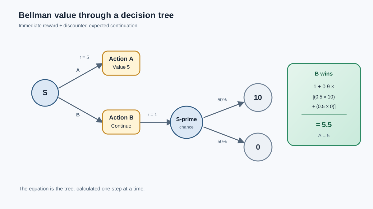
Imagine you are an agent standing at a starting state. Call it S. From S, you can pick one of two actions: A or B.
Here is what happens with each choice:
- If you choose A, you get a reward of 5 immediately. Then the episode ends.
- If you choose B, you get a reward of 1 immediately. Then you move to a next state, S′, with 50% probability you get an additional reward of 10, and with 50% probability you get nothing more.
Let me lay that out as a small tree:
                S
               / \
         action A action B
          /          \
      reward 5      reward 1
                       |
                      S'
                     /   \
                50% /     \ 50%
                   /       \
              reward 10   reward 0
Now, what is the value of being in state S?
If you choose A, the answer is easy. You get 5 and the story ends. The value of choosing A is 5.
If you choose B, you get 1 right away. Then you face a 50/50 gamble: half the time you collect 10 more, half the time you collect 0. The expected value of that gamble is:
(0.5 × 10) + (0.5 × 0) = 5
So the total value of choosing B is the immediate reward plus the expected continuation:
1 + 5 = 6
Here is what just happened. The value of choosing B was not a single reward. It was a weighted average of everything that follows—the guaranteed 1 now, plus the uncertain 10-or-0 later. That is the core insight: value is not one reward. It is a prediction about the future.
If you are trying to maximize expected reward, action B wins. Its value is 6, which beats action A's 5.
Knowledge check
Check your understanding
Answer this question before you continue.
From branch values to the Bellman equation
Now let me translate that hand calculation into the formal structure of the Bellman equation in reinforcement learning.
There is one piece I left out of the tree example: the discount factor, usually written as the Greek letter gamma (γ). The discount factor is a number between 0 and 1 that says how much you care about future rewards compared to immediate ones.
Why discount at all? Because a reward you get later is less valuable than the same reward you get now. It is delayed, it is less certain, and while you wait for it, other things could happen. A discount factor of 0.9 means a reward one step in the future is worth 90% of its face value to you right now. Two steps out, it is worth 0.9 × 0.9 = 81%.
In the tree example, I used no discounting—effectively γ = 1. Let me redo the calculation with γ = 0.9 to show how the discount factor enters.
For action B:
- Immediate reward: 1
- Expected continuation: (0.5 × 10) + (0.5 × 0) = 5
- Discounted continuation: 0.9 × 5 = 4.5
- Total value: 1 + 4.5 = 5.5
The value dropped from 6 to 5.5 because the future reward is now worth slightly less to you in the present.
Here is the general shape of what we just did:
Value = immediate reward + discount factor × expected value of what comes next
That is the Bellman equation. But to write it precisely, we need to name which value we are talking about. The tree gave us two different kinds of quantity, and confusing them is one of the most common beginner traps.
Action values vs. state values
When we calculated the value of choosing B, we were computing what is called an action value, written Q(s, a). It answers the question: How good is it to take this specific action from this state?
For the tree, the action values are:
Q(S, A) = 5
Q(S, B) = 1 + γ × [(0.5 × 10) + (0.5 × 0)]
With γ = 0.9, that gives Q(S, B) = 5.5.
A state value, written V(s), is a different object. It answers the question: How good is it to be in this state overall? The answer depends on what you do next. If you follow a fixed rule for choosing actions—called a policy, written π—then V(s) averages over whatever actions that policy might pick. If you act optimally, V(s) takes the best action instead.
So the relationship between the two is simple:
- Under a policy π: V^π(s) = expected value of Q^π(s, a), averaged over the actions π chooses.
- Acting optimally: V*(s) = the maximum of Q*(s, a) over all available actions.
In the tree, if your policy is "always choose B," then V(S) = Q(S, B) = 5.5. If you act optimally, V(S) = max(5, 5.5) = 5.5. The numbers happen to match because B is the better action—but the meaning is different, and that difference matters when you compare actions.
The compact form
With that distinction in place, here is the Bellman equation for an action value under a fixed policy:
Q^π(s, a) = expected immediate reward + γ × expected value of the next state
And here is the optimality version, which uses a max because the agent gets to choose the best action at every step:
Q*(s, a) = expected immediate reward + γ × expected value of the best next action
Every symbol in these equations maps back to a piece of the tree you already computed by hand. The equation is not a magic formula. It is a prediction rule that says what value should be if the future unfolds as expected.
Knowledge check
Check your understanding
Answer this question before you continue.
The expectation equation vs. the optimality equation
Beginners often hit a wall here because there are two versions of the Bellman equation floating around, and they look almost identical. The difference is one word: expectation versus optimality.
The Bellman expectation equation answers this question: If I follow a fixed policy—a fixed rule for choosing actions—what value should I expect?
In the tree example, imagine your policy is "always choose B." The expectation equation averages over whatever that policy does. Since the policy always picks B, you average over the outcomes that follow B. The value you get is the one we computed: immediate reward plus discounted expected continuation, following the policy's choices.
The Bellman optimality equation answers a different question: If I get to choose the best action at every step, what is the most value I can possibly get?
Now the max appears. Instead of averaging over what your policy does, you look at every action and pick the one with the highest expected outcome. In the tree, that means comparing action A's value of 5 against action B's value of 5.5 (with γ = 0.9), and choosing B because it is larger.
The structural difference between the two equations is exactly that max. The expectation equation averages over the policy's choices. The optimality equation maximizes over them.
| Bellman expectation equation | Bellman optimality equation | |
|---|---|---|
| Question it answers | How good is this state under my current policy? | How good is this state if I act optimally? |
| What it does with actions | Averages over what the policy does | Picks the action with the highest value |
| Where the max appears | Nowhere | At every choice point |
| When you use it | To evaluate a policy | To search for the best policy |
Both versions share the same recursive structure: one-step reward plus discounted continuation. The only question is whether "continuation" means what my policy will do or what the best possible choice would do.
Knowledge check
Check your understanding
Answer this question before you continue.
Where the mental model helps and where it breaks down
The decision tree is an honest mental model. It shows you exactly what the equation means, and you can verify every number by hand. But it is worth being clear about where the model stops matching reality.
The tree works because it is small, known, and finite. You know every branch, every probability, every reward. Real reinforcement learning environments are not like that. They are large, unknown, and often continuous. The agent does not receive a diagram of possible futures. It receives one experience at a time: a state, an action, a reward, a next state.
The tree also assumes that the current state contains the information you need to predict what matters next. Real environments may hide relevant details, and the probabilities shown in the tree are not handed to a learning agent—it must estimate them from experience.
This changes the practical meaning of the equation. The "prediction" is no longer something you read off a known tree. It is an estimate the agent updates over time as it collects more data.
The equation stays the same in spirit. But the continuation term becomes a guess that gets revised, not a fact that gets looked up.
This is the bridge to why algorithms like Q-learning exist. Q-learning takes the Bellman structure—one-step reward plus discounted continuation—and learns the continuation prediction from data instead of reading it off a known model. The equation is the target the algorithm keeps trying to hit. Every update is a small correction toward making the prediction self-consistent.
A quick check you can run yourself
Let me give you one small variation on the tree so you can test whether the recursive reading has stuck.
Same starting state S. Same two actions. But now the rewards have changed:
- Action A: immediate reward of 8. Episode ends.
- Action B: immediate reward of 2. Then you move to S′. With 50% probability you get 12 more; with 50% probability you get 0.
Use a discount factor of γ = 0.9. Which action has higher value?
Here is the calculation:
- Value of A: 8
- Value of B: 2 + 0.9 × [(0.5 × 12) + (0.5 × 0)] = 2 + 0.9 × 6 = 2 + 5.4 = 7.4
Action A wins this time, even though B offers a chance at a larger future payoff. The immediate reward gap is too large, and the discount factor shrinks the future reward enough that the gamble no longer pays.
Notice what you just did. You did not memorize a formula. You read the situation as immediate reward plus discounted continuation, applied the same rule at each step, and compared the results. That is the Bellman equation in action.
One mistake to watch for: discounting the immediate reward. The discount factor applies to the continuation, not to the reward you collect right now. A common arithmetic slip is writing 0.9 × 2 instead of 2 for action B's immediate reward. The immediate reward is already in the present—it does not get discounted.
Another trap: choosing the action with the larger possible payoff instead of the larger expected payoff. Action B offers a chance at 12, but that chance is only 50%. The expected continuation is 6, not 12. Always compare expected values, not best-case outcomes.
The natural next step is to take this recursive reading and apply it to value functions more broadly—and then to the learning algorithms that refine value estimates from experience. When you meet Q-learning or temporal-difference learning, you will recognize the same structure underneath: every update is the agent trying to make its prediction consistent with the one-step reward plus the discounted continuation it actually observed.
Knowledge check
Final check
Finish the article by checking the ideas you just learned.
References
Research updated Sep 9, 2026


