
Why Bellman Updates Converge: A Fixed-Point Mental Model for RL
Value iteration is not a loop that guesses better. It is a machine that shrinks the distance between any two value estimates by a factor of gamma on every…

Key topics
Value iteration is not a loop that guesses better. It is a machine that shrinks the distance between any two value estimates by a factor of gamma on every pass.
If you have traced a Bellman backup through a small environment, you know the mechanics: take the current estimate, compute one-step reward plus discounted continuation, and write the result back. You can perform that update in your sleep. But there is a moment when the tracing stops being enough. You run the loop, the numbers change, and somehow they settle. Why do they settle instead of oscillating, drifting, or landing on the wrong answer?
That question is the difference between operating the algorithm and understanding it. Let's replace the magic with a mechanism you can watch in the numbers.
The Question Behind the Backup
Here is the gap most beginners hit: a single Bellman update is easy to justify. You are correcting one estimate using neighboring estimates. But a thousand updates feel different. Each pass changes every value, which changes the inputs to the next pass, which changes every value again. It looks like a system that could reasonably wobble forever.
The surprise is that it cannot. The Bellman equation converges because of a property that has nothing to do with the specific rewards in your environment and everything to do with the structure of the update itself.
The core claim is simple: the exact Bellman operator shrinks the worst disagreement between any two value functions by a factor of gamma. If two estimates disagree by at most 10 anywhere and gamma is 0.9, the next pass brings their worst disagreement to at most 9. Then 8.1. Then 7.29. The process is not hoping to find the right answer. It is being dragged toward it, and the drag gets weaker as the disagreement shrinks.
Before we can see why, we need to change what we are looking at.
What a Bellman Operator Actually Does
When you first learn value iteration, you think in terms of individual states: update V(s₁), then V(s₂), then V(s₃). That framing is useful for tracing, but it hides the structure that makes convergence work.
Step back and look at the whole value function at once. A value function is just a table of numbers, one per state. A Bellman backup takes that entire table and produces a new table. That makes the update a single operation on the whole function — a machine that consumes one value function and outputs another.
In reinforcement learning, we call that machine the Bellman operator. It is a function that maps value functions to value functions. Value iteration is not a sequence of per-state updates. It is the repeated application of one operator:
V_new = T(V_old)
where T is the Bellman operator. Apply it once, you get a new estimate. Apply it again, you get another. The whole loop is just T acting over and over.
Now the key question becomes: what happens when T meets the true value function?
The Bellman equation says that the true value function satisfies V = T(V). Apply the operator to the true values, and the output is identical to the input. The true value function is a fixed point of the operator — a point where the machine's output equals its input. The operator looks at the true values, computes one-step reward plus discounted continuation, and gets back exactly what it started with. No correction needed, because there is no error to correct.
That gives us a target. The question is why repeated application of T pulls any starting guess toward that fixed point rather than somewhere else.
Knowledge check
Check your understanding
Answer this question before you continue.
The Shrinking-Distance Intuition
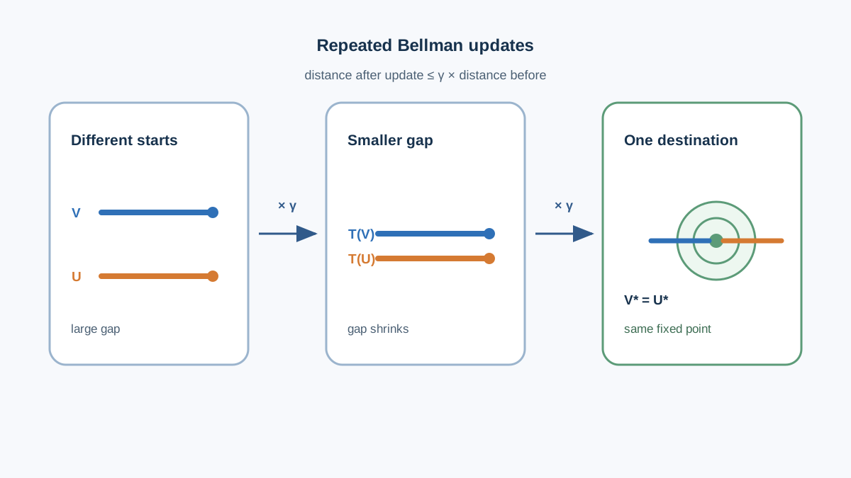
Here is where the mechanism becomes visible. Take two different value functions, call them V and U. They disagree about some states — maybe badly. Apply the Bellman operator to both, producing T(V) and T(U). How much do the outputs disagree?
Write out what the operator does. For each state, it computes the reward plus the discounted value of the next state. When you compare T(V) and T(U) at the same state, the reward term is identical in both. It cancels. What remains is the difference between V and U at the next state, multiplied by gamma.
The worst disagreement between the two outputs is therefore gamma times the worst disagreement between the two inputs. If V and U differ by at most 10 anywhere, then T(V) and T(U) differ by at most 10γ anywhere. With gamma below 1, the operator has squeezed the gap.
This is the property that makes convergence inevitable. Imagine two completely different starting guesses. Run the operator on both. The gap between them shrinks by gamma. Run it again, and it shrinks again. After n passes, the gap is at most γⁿ times the original gap. The two estimates are being forced together, and the force never reverses.
Since the true value function is a fixed point, you can use it as one of the two functions. Compare any starting guess against the truth. Each pass shrinks the distance to that fixed point by gamma. The estimate is not wandering. It is converging geometrically toward the one function the operator leaves unchanged.
This property has a name — contraction — but the name is just a label for what you just watched. An operator is a contraction when applying it to any two inputs brings them closer by a fixed factor. The Bellman operator is a contraction with factor gamma. That single fact guarantees both that a fixed point exists and that repeated application reaches it, regardless of where you start.
Note: The contraction claim is about the largest absolute difference across all states — the technical term is the sup norm. When we say the worst disagreement shrinks by gamma, that worst case is measured over every state in the environment. This matters because a contraction guarantee must hold everywhere, not just on average.
One clarification before moving on: the contraction inequality is an upper bound, not an exact prediction. Each pass shrinks the worst disagreement to at most gamma times its previous value. In practice, the gap often shrinks faster. The guarantee is that it never shrinks slower.
Knowledge check
Check your understanding
Answer this question before you continue.
Why Discounting Is the Engine
Notice what made the argument work: the reward terms canceled, and the remaining difference was multiplied by gamma. If gamma were 1, the operator would not shrink anything. It would preserve the worst disagreement forever, and the convergence argument would collapse.
This is why discounting is not just a modeling preference. It is the engine of the entire fixed-point argument. The discount factor is the contraction constant. It determines how fast the distance shrinks, and whether it shrinks at all.
The practical consequence is visible in convergence speed. With gamma = 0.9, each pass shrinks the worst distance to 90% of its previous value. After about 22 passes, the gap is down to roughly a tenth of where it started. With gamma = 0.99, the same reduction takes about 230 passes. The convergence is still guaranteed, but you can feel the slowdown. The closer gamma gets to 1, the closer the operator gets to preserving distance instead of shrinking it.
At gamma = 1 in an infinite-horizon setting, the clean guarantee can fail entirely. Returns can be infinite, the value function can be ill-defined, and the contraction argument no longer applies. The boundary is not a technicality. It is the exact point where the machine stops being a distance-shrinker.
Knowledge check
Check your understanding
Answer this question before you continue.
Where This Mental Model Holds — and Where It Breaks
The fixed-point story is clean, powerful, and easy to over-apply. So let's be precise about where it lives.
The guarantee applies to tabular value iteration and policy evaluation on a known, discounted MDP with exact backups. You have a complete model of transitions and rewards. You update every state using exact expectations. The operator is applied exactly, and the contraction argument holds without qualification.
The moment you change any of those conditions, the story weakens. But it weakens in different ways depending on what you break:
| Setting | What changes | Does the contraction proof survive? |
|---|---|---|
| Exact backups on a known MDP | Nothing — the operator is applied exactly | Yes, fully |
| Sample-based updates (TD learning) | Each update carries sampling noise instead of exact expectations | Requires separate stochastic-approximation conditions; the clean guarantee does not transfer automatically |
| Function approximation | The operator's output may not be representable by your function class | No — the operator may map outside the space it acts on |
| Deep RL with neural networks | Adds moving targets, optimization dynamics, and representation drift on top of approximation | No — the tabular theorem does not apply |
Replace exact backups with samples, and you are no longer applying the Bellman operator. You are applying a noisy approximation of it. Temporal difference learning uses single transitions instead of full expectations, which means each update carries sampling error on top of the contraction. The clean guarantee does not transfer automatically.
Replace the tabular value function with a function approximator, and the problem gets worse. The Bellman operator may produce a value function that your function class cannot represent. The operator maps the true function space into itself, but it may not map your neural network family into itself. The contraction argument assumes the operator acts on the same space throughout. When the function class cannot express the operator's output, the fixed-point reasoning no longer applies directly.
This is why deep RL agents can diverge or plateau even when the underlying Bellman operator is perfectly well-behaved. The clean theory and the messy practice are answering different questions. The theory says the exact operator converges. Practice says that approximate operators on restricted function classes need additional machinery — target networks, replay buffers, careful step sizes — to stay stable.
Common mistake: Do not assume that target networks or replay buffers "restore" the contraction proof. Those engineering devices address specific failure modes in deep RL, but they do not recreate the exact-operator conditions that make the fixed-point argument clean. The tabular theorem and the deep RL practice are different regimes, not two versions of the same guarantee.
Here is my rule of thumb: trust the fixed-point intuition when you are working with small tabular experiments and when you want to understand why value iteration works at all. Do not expect it to explain deep RL convergence. The mental model tells you what the exact process does. It does not tell you what happens when you break the exactness.
Knowledge check
Check your understanding
Answer this question before you continue.
A Mental Model You Can Carry Forward
Compress the whole argument into one sentence: value iteration is a machine that shrinks the worst distance between any two value functions by gamma on every pass, so it drags every starting guess toward the one function the operator leaves unchanged.
If you want to feel this rather than just follow it, run the experiment. Take a tiny environment — a three-state chain is plenty. Initialize the value function two different ways: all zeros in one run, all tens in another. Run value iteration on both with synchronous, exact sweeps, and watch the estimates meet.
After each sweep, measure the largest absolute difference between the two tables. Compare it with gamma times the previous gap. You should see the gap shrink to at most that bound — often faster, never slower. Watching two arbitrary guesses get pulled to the same answer is the fastest way to make a fixed point feel real.
One caveat: two runs agreeing with each other is evidence of stability, not direct proof that either table is optimal. The contraction guarantees the runs converge together; the Bellman equation guarantees that the point they meet at is the true value function. Both halves matter.
The natural next question is where this clean picture breaks: what happens when you replace exact backups with samples, or tables with neural networks? That is the bridge into temporal difference learning and deep RL, where the contraction argument stops being the whole story and starts being the background against which real algorithms struggle. The fixed-point model you have now is the foundation for understanding why those struggles exist at all.
Knowledge check
Final check
Finish the article by checking the ideas you just learned.
References
Research updated Sep 9, 2026


