Markov Decision Processes: The Formal Map Behind Reinforcement Learning

The agent-environment loop feels simple until you try to make an algorithm learn. Then the loop stops being enough. The agent needs to know what it can see, what it can do, and what it should expect in return. The environment needs to know how to respond. Both sides need to agree on what counts as a good outcome over time.

That agreement is a Markov decision process—the formal map that turns "the agent tries things" into a precise, computable problem definition. Once you can read that map, you can see exactly what any reinforcement learning algorithm is trying to solve. Just as important, you can see when the map itself is missing a piece.

From Intuition to a Formal Map

Think of the agent-environment loop as a conversation. At each step, the agent says, "Here is what I observe, and here is what I choose to do." The environment replies, "Here is your reward, and here is your new situation." Intuition tells you the conversation exists. But algorithms do not run on intuition. They need a contract that says exactly what each side guarantees.

A Markov decision process is that contract. It is the standard way to describe a sequential decision problem in reinforcement learning, and it answers one question: what does the agent need to know to make good decisions over time, not just in this moment?

The answer comes in five parts: states, actions, transitions, rewards, and a discount factor. Together they form the MDP tuple, usually written as (S, A, P, R, γ). That notation looks intimidating until you realize each piece has a concrete job.

The Five Ingredients of an MDP

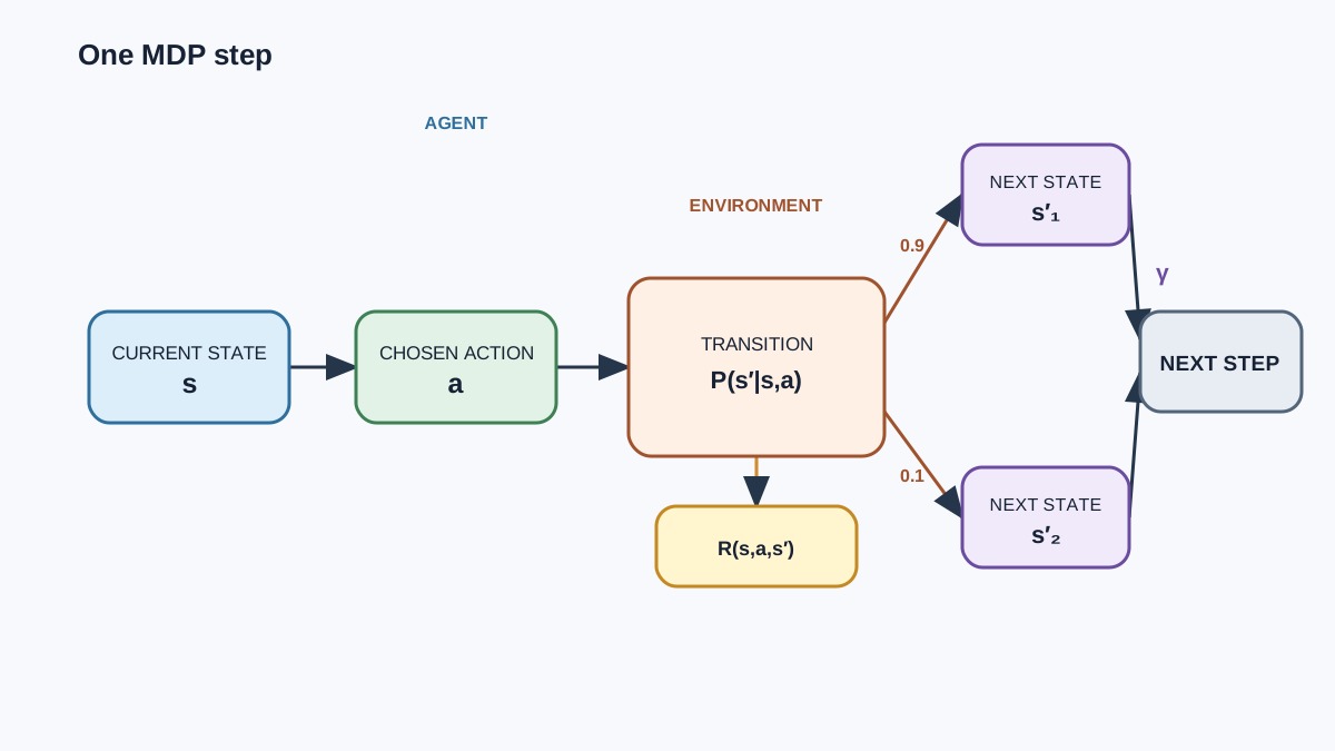
To make this concrete, let's carry one small environment through the whole article. Imagine a robot delivery cart in a warehouse with three loading zones. The cart can be at zone A, zone B, or zone C. It carries packages that need to reach specific zones, and its battery drains as it moves.

States are the situations the agent can be in. In the warehouse, a state might be "at zone A with two packages and 80% battery." The state needs to contain whatever information the agent requires to decide well. If the cart does not know its battery level, it cannot choose between "keep delivering" and "return to charge." The set of all possible situations is the state space, S.

Actions are the choices available in each state. The cart can drive to another zone, pick up a package, drop one off, or head to the charging station. Some actions may be forbidden in some states: you cannot drop off a package you are not carrying. The set of legal actions in a state is often written A(s), and the full set of actions across all states is A.

Transition probabilities are the environment's rules for where an action leads. This is where the MDP stops feeling like a deterministic flowchart. In the warehouse, the cart might command "drive to zone B," but wheels slip, obstacles appear, and the cart ends up at zone C instead. The transition function P(s′ | s, a) says: given that the agent was in state s and took action a, the probability of landing in state s′ is some number between 0 and 1. For each state-action pair, those probabilities must sum to 1—something has to happen.

This is the piece beginners most often forget. They build environments as if every action had one guaranteed outcome. Real environments are noisy. The transition function is where that noise lives.

Rewards are the immediate signal the agent receives after taking an action. In the warehouse, the cart gets +10 for a successful delivery and −1 for every move, to encourage efficiency. The reward function R(s, a, s′) says how much feedback the agent gets for this one step. Keep it separate from the long-term return the agent is really optimizing. A reward is a single data point; the return is the accumulated story.

The discount factor γ (gamma) is a number between 0 and 1 that answers a quiet question: how much should the agent care about the future? A reward now is worth more than the same reward later, because later rewards are less certain and because waiting costs something. With γ close to 1, the agent treats distant rewards as nearly as valuable as immediate ones. With γ close to 0, the agent becomes short-sighted, chasing whatever reward is closest.

Here is the practical way to read the discount factor: it shapes priorities. If your agent should plan several steps ahead, keep γ high. If the environment changes fast and distant predictions are unreliable, lower it. The discount factor is not a knob for fixing a broken reward design—it is a statement about how much the future should matter.

Now the tuple (S, A, P, R, γ) has meaning. States say where the agent can be. Actions say what it can do. Transitions say what happens when it acts. Rewards say what it feels immediately. Discounting says how much the future counts. Together, they define the entire problem.

A Worked Example: Reading the Map Back

Definitions only become tools when you see them constrain one another. So let's build a deliberately tiny version of the warehouse and write down every piece.

Keep the cart at two zones, A and B. The cart carries at most one package. The state needs two facts: location and whether the cart is loaded. That gives four states:

• A, empty
• A, loaded
• B, empty
• B, loaded

Legal actions depend on the state. From A, empty, the cart can drive to B or pick up a package. From A, loaded, it can drive to B or drop off. The same pattern holds at zone B.

Now add noise. When the cart commands "drive to B," it arrives at B with probability 0.9 and stays at A with probability 0.1. The cart's wheels slip. That single number is the transition probability, and it changes everything: the agent can no longer assume its command will be executed perfectly.

Rewards follow the outcome. A successful delivery earns +10. Every move costs −1. Picking up a package costs nothing. If the cart tries to drop off while empty, that action is simply not legal—it is excluded from A(s).

Finally, set γ = 0.95 and declare the episode terminal when a delivery completes. The cart starts at A, empty.

Read that specification back in plain language: the cart knows where it is and whether it is carrying anything. It can move, pick up, or drop off, subject to what it is holding. Movement is noisy. Deliveries pay well, movement costs a little, and the future matters almost as much as the present. That is a complete Markov decision process—small enough to hold in your head, precise enough that an algorithm could optimize it.

Notice what the formal specification caught. Writing down legal actions forced you to handle the "drop off while empty" case. Writing down transitions forced you to decide how reliable movement really is. Writing down rewards forced you to state what a delivery is worth relative to the cost of moving. The map does not just describe the problem. It exposes the places where your intuition was vague.

The cart is at A, empty, and can drive to B or pick up a package.

What the Markov Property Actually Claims

Here is the assumption that makes all of this tractable: the next state depends only on the current state and the action just taken. Not on everything that happened before. Not on the path that led here. Just on where you are now and what you just did.

That claim is the Markov property, and it is a powerful simplification. If the state captures everything relevant about the past, the agent can forget history entirely and still make optimal decisions. The current state is a sufficient summary of everything that came before it.

To see why this matters, imagine the cart arrives at zone B. If the state is just "at zone B," the agent has no idea whether it arrived with a full package load or an empty rack. The same visible situation hides two very different underlying conditions, and the right action depends on which one is true. The naive state is not Markovian: the next state and the best decision both depend on history the agent cannot see.

The repair is straightforward. Add the missing information to the state. Instead of "at zone B," use "at zone B carrying two packages." Now the state contains everything the agent needs to decide, and the Markov property holds again. The agent can forget how it got here because the state itself remembers what matters.

This is the habit that separates people who can read about reinforcement learning from people who can actually formulate a problem an algorithm can solve: treating the state as a design decision, not a given.

When the Markov Assumption Breaks

The Markov property fails in recognizable ways, and once you know the symptoms, you can diagnose them before your agent starts behaving erratically.

The most common failure is partial observability. The agent only sees part of the environment, so the same observation can hide different underlying situations. The cart's camera sees zone B, but it cannot see whether the package shelf is stocked. Two different true states produce the same observation, and the agent cannot tell them apart.

Another failure is missing memory. The state lacks something that matters, like velocity or the effect of a previous action. A robot that only tracks position but not momentum will make the same decision at the same spot whether it is moving slowly or fast—and get very different results.

The observable symptom is inconsistency. The agent behaves erratically because the same state leads to different outcomes depending on hidden factors. If your agent sometimes succeeds and sometimes fails from what looks like the same situation, suspect the state before you suspect the learning algorithm.

The standard repair is to enrich the state with the missing variable. Add velocity. Add the last action. Add a short history buffer when a single snapshot is not enough. The Markov property is not a fact about the world; it is a property of your state representation. You can often design your way back into it.

There is a boundary worth naming. When the true state is genuinely unrecoverable—when no amount of state engineering can capture what the agent needs—the problem stops being a clean MDP and becomes a partially observable Markov decision process (POMDP). That is a distinct topic with its own methods, and you should flag it rather than pretending the MDP framing still holds.

From MDP to a Policy: What the Agent Is Searching For

Once the MDP is fixed, the agent's job becomes clear: find a policy. A policy is a decision rule, a mapping from states to actions. A deterministic policy says, "In this state, do that." A stochastic policy says, "In this state, choose among these actions with these probabilities."

The MDP defines the search space and the objective. The policy is what the agent is looking for. The agent wants the policy that maximizes expected discounted return—the sum of rewards over time, with future rewards weighted by γ.

This is the bridge to everything that comes next. Once the MDP is in place, value functions and Bellman reasoning become the tools for evaluating how good a policy is and improving it. But those tools only work because the MDP gave them a well-defined problem to solve. Get the map wrong, and no amount of clever value estimation will save you.

Common Mistakes When Building an MDP

Beginners tend to make the same four mistakes when translating a real environment into an MDP. Catch them before they reach an algorithm.

Mistake 1: Treating transitions as deterministic. If you assume every action has one guaranteed outcome, you will be surprised when the real environment is noisy. The fix is to ask what could actually happen after each action, not just what you hope will happen.

Mistake 2: Leaving information out of the state. This silently breaks the Markov property. The agent cannot use what it does not have. The fix is to test your state by asking: if the agent knew only this state and not the history, could it still make the right decision?

Mistake 3: Conflating reward with return. A reward is one step of feedback. The return is the accumulated, discounted sum. Beginners design a reward signal without thinking about how it accumulates, and the agent optimizes the accumulation in ways the designer never intended. The fix is to simulate your reward design and watch what behavior it encourages over many steps, not just one.

Mistake 4: Ignoring terminal states or abusing the discount factor. Some environments have a clear end—the game finishes, the delivery completes, the episode stops. If you forget terminal states, your agent keeps acting in a world that should have ended. And if you lower γ to fix a reward problem, you are treating a symptom while the cause remains.

The Practice Move That Makes This Stick

Here is where the formalism pays off. Take a small environment you already understand—a game, a workflow, a simple automation—and write down its five MDP ingredients. What are the states? What actions are available in each? What outcomes can each action produce, and with what probability? What reward does each step deliver? How much should the future matter?

Then do the harder step. Deliberately test whether the Markov property holds. Find the state that hides something the agent needs. Repair it by adding the missing information. Watch the problem become solvable.

That habit—formulating the map before running the algorithm—is the real skill. The MDP is not academic decoration. It is the contract that lets you know exactly what problem you are solving, where the assumptions hold, and where they need repair. Build that habit now, and every value function, policy gradient, and Bellman update you learn next will have a solid map to operate on.

References

Research updated Sep 9, 2026