Bellman Backups and Dynamic Programming for Reinforcement Learning

A Bellman equation states a consistency condition. A Bellman backup is the mechanical step that enforces it. The difference between reading an equation and watching numbers converge is the difference between knowing a rule and running it.

If you have seen the Bellman equation before, you know its shape: the value of a state equals the immediate reward plus the discounted value of whatever comes next. Clean, compact, and completely static. Nothing moves. No numbers change. It is a statement about what must be true when values are correct—not a recipe for making them correct.

This article closes that gap. You will trace a Bellman backup through a tiny environment, watch value estimates ripple backward from rewards, and see how three dynamic programming algorithms—policy evaluation, policy improvement, and value iteration—turn one repeated update into a complete solution method.

From Bellman Equation to Bellman Backup

Here is the bridge from equation to algorithm. The Bellman equation says:

The value of a state = immediate reward + discounted value of what comes next.

A Bellman backup treats the right-hand side of that equation as an update rule. Take your current estimate for a state, compute reward-plus-next-value using the estimates of neighboring states, and write the result back. That single operation—read, compute, write—is a backup.

Why is one pass never enough? Because the values depend on each other. When you update state A, you change the estimate that state B will use in its next update. And when B changes, it feeds back into A. The updates must ripple through the state graph many times before every estimate settles into agreement.

Let's make that concrete with the smallest environment that shows the mechanism: a three-state chain.

A Worked Trace: Three States and a Terminal Reward

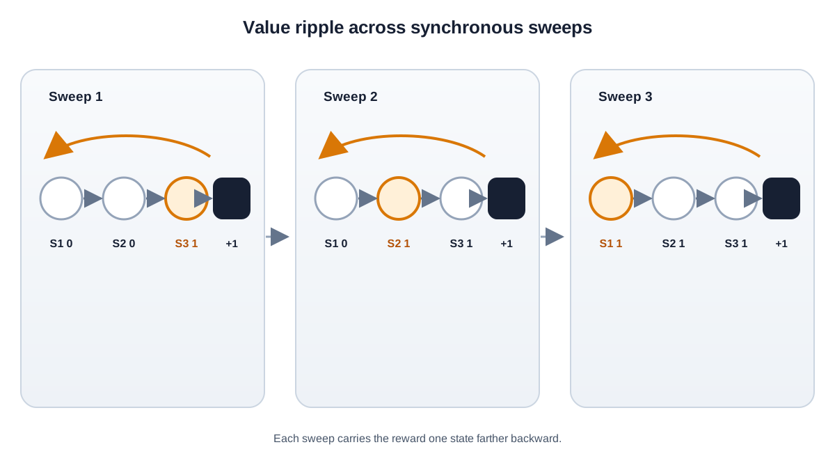
Imagine three states in a row—call them S1, S2, and S3. From S1 you move to S2. From S2 you move to S3. From S3 you move to a terminal state and collect a reward of +1. No other rewards exist, and the discount factor is 1 for simplicity.

Initialize every state's value to 0. Now apply the backup. For each state, the new value is:

reward from leaving this state + value of the state you land in

Here is what one synchronous sweep produces. A synchronous sweep means every state is updated using values from the previous table, so the order of updates does not matter.

State	Old value	Backup calculation	New value
S1	0	0 + value(S2) = 0 + 0	0
S2	0	0 + value(S3) = 0 + 0	0
S3	0	1 + value(terminal) = 1 + 0	1

Only S3 learned anything. It sits one step before the reward, so its backup can see it. S1 and S2 look ahead to neighbors that are still zero, so their estimates stay flat.

Run a second sweep.

State	Old value	Backup calculation	New value
S1	0	0 + value(S2) = 0 + 0	0
S2	0	0 + value(S3) = 0 + 1	1
S3	1	1 + value(terminal) = 1 + 0	1

Now S2 moves. Its backup sees S3's nonzero value and adopts it. Run a third sweep, and S1 finally updates to 1 as well.

That is the core intuition: each backup propagates value one step closer to the states that need it. The reward information travels backward through the state graph like a wave, and each full sweep pushes the wave one state farther.

Note: If you implement this with in-place updates—where each state immediately overwrites its old value and later states in the same sweep read the new number—values can propagate farther in a single pass. The intermediate tables will differ, but the final converged values will not. The synchronous version is easier to trace by hand, which is why this example uses it.

What Dynamic Programming Actually Requires

Dynamic programming solves the planning problem. It assumes you already have a complete model of the environment: the transition probabilities between states and the reward structure. No exploration, no trial and error, no learning from experience. You hand DP the rules of the game, and it computes the optimal policy by reasoning through them.

This is the sharp boundary between DP and model-free reinforcement learning. DP uses the known model to calculate. Model-free methods estimate from sampled experience. One reads the map; the other walks the streets and remembers what it finds.

The practical consequence is immediate. DP shines on small, known, tabular MDPs where you can enumerate every state and compute every transition. It becomes infeasible as state spaces grow, because each sweep touches every state and every action. If your environment has millions of states, exact DP is out of reach.

My rule of thumb: use DP when you can write down the complete environment dynamics and the state space is small enough to iterate over. Use model-free methods when the agent must discover the environment through interaction or when the state space defeats exhaustive sweeps.

Policy Evaluation: Turning a Fixed Policy into Numbers

Policy evaluation answers the prediction problem: given a fixed policy, what is the value of each state under that policy?

The algorithm is straightforward. Initialize all state values to zero. Then repeatedly sweep through every state, applying the Bellman backup for the current policy. For each state, compute the expected reward-plus-discounted-next-value under the actions the policy selects, and replace the old estimate with the new one. Stop when the largest change across any state falls below a small tolerance.

Return to the three-state chain, but now imagine the policy is not deterministic. Suppose from S2 the policy sometimes moves to S3 and sometimes wanders back to S1. The backup changes: instead of reading the value of one guaranteed next state, you average over the values of every possible next state, weighted by the policy's action probabilities and the environment's transition probabilities.

The shape of the update is the same—read neighbor values, compute, write back—but the computation now blends multiple futures. That is why the chain example above used a deterministic policy: it isolates the propagation mechanism from the averaging detail.

A common beginner mistake is expecting convergence in one pass. It will not happen. Values depend on other values, and those dependencies take multiple sweeps to resolve. Another mistake is confusing the value of the current policy with the optimal value. They coincide only when the policy you are evaluating is already optimal. Until then, policy evaluation tells you how good this policy is—not how good the environment can be.

Policy Improvement: Using Values to Pick Better Actions

Once you trust the value function for the current policy, you have a lever for improvement. At each state, ask a different question: which action produces the highest reward-plus-discounted-next-value?

That greedy step is policy improvement. If acting greedily with respect to the current value function improves the expected return at every state, the new policy is at least as good as the old one. And if the greedy policy is no better than the policy it came from, you have reached the optimum: a policy that is greedy with respect to its own value function is optimal.

The policy improvement theorem guarantees this convergence in the finite, tabular setting we are working in. It says that evaluating a policy, improving it greedily, and repeating will eventually reach an optimal policy. The proof matters less than the intuition: each improvement step either finds a strictly better policy or confirms that the current one cannot be beaten.

The mistake to avoid here is impatience. If you improve the policy before evaluation has converged, you are making decisions based on unreliable numbers. The values need to settle before they can be trusted as a basis for comparison.

Common mistake: Full convergence is not always required before every improvement step. Value iteration, which we turn to next, deliberately improves after a single sweep. The distinction is not "always evaluate fully" versus "never evaluate fully." It is a spectrum, and where you sit on it is a design choice.

Policy Iteration vs Value Iteration: Two Ways to Reach Optimality

Policy iteration and value iteration are the two classic control algorithms, and they differ in how they structure the evaluation-improvement loop.

Policy iteration alternates between two complete phases. First, fully evaluate the current policy until its value function converges. Second, improve the policy greedily with respect to those values. Repeat until the policy stops changing. Each outer cycle is expensive—full evaluation can take many sweeps—but the number of cycles is often small.

Value iteration fuses the two phases into a single update. Instead of evaluating a fixed policy to convergence, it applies one backup per state per sweep using the maximum over actions. The update asks: what is the best action here, and what is its reward-plus-next-value? Write that back. Repeat until the values stop changing. The result converges directly to the optimal value function, from which the optimal policy falls out by taking the greedy action at each state.

Watch how the backup differs from policy evaluation. In the three-state chain, policy evaluation under a deterministic policy reads the value of the one action the policy selects. Value iteration reads the values of all available actions and keeps the largest. That max is the entire difference between evaluating a given policy and searching for the best one.

Conceptually, value iteration is policy iteration where evaluation is cut short to a single sweep. That is the spectrum between them: you can run any number of evaluation sweeps between improvement steps, and the two extremes are full evaluation (policy iteration) and one sweep (value iteration).

	Policy Iteration	Value Iteration
Structure	Full evaluation, then improvement	Single backup with max per sweep
What converges	The policy	The value function
Outer cycles needed	Usually fewer	Usually more
Cost per outer cycle	Higher	Lower
When to prefer	Good initial policy; evaluation is cheap	Simplicity and ease of implementation matter

One caution about that table: the iteration counts are not directly comparable. A single policy-iteration cycle may contain many internal evaluation sweeps, while one value-iteration sweep is a single pass over the states. "Fewer iterations" for policy iteration means fewer policy changes, not fewer total updates.

My practical preference: implement value iteration first. It is simpler, requires less bookkeeping, and converges reliably on small environments. Policy iteration becomes attractive when you have a good initial policy and evaluation is inexpensive, because it can reach the optimum in fewer improvement cycles.

Common Mistakes When Learning Dynamic Programming

Four failure modes trip up nearly every beginner. If your output looks wrong, trace which one you violated.

Mistake 1: treating the Bellman equation as a formula to memorize. The equation is a consistency condition. The backup is the update that enforces it. Memorizing the equation without running the update gives you a static fact, not a working algorithm.

Mistake 2: confusing the value of the current policy with the optimal value. They are different quantities that happen to share notation. The value of the current policy tells you what happens if you follow that policy forever. The optimal value tells you what happens if you act optimally. They coincide only at the optimum.

Mistake 3: forgetting that DP needs the full model. If your agent must explore to discover rewards and transitions, DP cannot help. You need a model-free method. DP is a planning tool, not a learning tool.

Mistake 4: skipping the max over actions in value iteration. This is the silent killer. If you apply the policy evaluation backup—averaging over the policy's actions—instead of the max over actions, you are no longer doing value iteration. You are evaluating whatever implicit policy your averaging represents. The max is what pushes values toward optimality.

Where Dynamic Programming Fits in Your RL Toolkit

Dynamic programming is the clean, model-based foundation that later sample-based methods relax. Monte Carlo methods replace computed expectations with sampled returns. Temporal difference learning replaces full sweeps with single-step updates from experience. Q-learning replaces the known model with bootstrapped estimates from observed transitions.

But the backup idea survives every one of those changes. When you update a Q-value in Q-learning, you are performing a backup—just one that uses a sampled next state instead of an expectation over all possible next states. Master the backup in its clean DP form, and you will recognize its descendants everywhere.

Here is your next move. Implement value iteration on a small known grid world—something like a 4x4 grid with a goal state and a penalty per step. Print the value table after every sweep. Watch the reward information propagate one cell per sweep, exactly like the three-state chain. Then change the reward structure: make one corner costly, move the goal, add a wall. Observe how the optimal policy shifts in response. That experiment will make the mechanism visible in a way that reading about it never will.

The durable takeaway is this: a Bellman backup is a small, repeatable update. The equation states what correct values look like. The backup is how you get there—one sweep at a time, pushing value backward through the state graph until the numbers agree.

References

Research updated Sep 9, 2026