Policy Improvement and Generalized Policy Iteration in Reinforcement Learning

You can compute value estimates. You can trace a Bellman backup through a small grid. But if someone asked you to explain how those numbers actually change what the agent does next, would you have a crisp answer?

That gap—between knowing how good a state is and deciding which action to take—is where most beginners get stuck. The missing piece is policy improvement in reinforcement learning: the step that turns value information into better decisions. And once you see that step clearly, the entire control loop behind most RL methods snaps into focus.

The Gap Between Knowing Values and Choosing Actions

Here is the situation that trips up many newcomers. You have spent time computing value estimates for every state in a small environment. You have a table of numbers that tells you, under your current policy, how much discounted future reward the agent can expect from each state. You feel ready to solve the problem.

Then you realize the table does not tell you what to do.

A value estimate describes a state under a policy. It does not recommend an action. If your agent is in state s and your policy says "go left," but the value table suggests that being in the state you would reach by going right is worth more—so what? Nothing in the value function itself tells you to switch. Something else has to do that work.

That something else is the improvement step. It is the decision rule that looks at value information and changes which action the policy recommends. Without it, you have a measurement with no mechanism for acting on it.

If you need a refresher on what value functions predict or how Bellman backups work, those are worth revisiting first. The short version: V(s) tells you the expected return from state s under a fixed policy, and Q(s, a) tells you the expected return from taking action a in state s and then following that policy. This article is about what happens after you have those estimates.

What Policy Improvement Actually Does

Policy improvement is a greedy decision rule. For each state, you compare the action values of the available actions and switch the policy to the action with the highest expected return.

That is the whole mechanism. It is almost embarrassingly simple. But it has a strong theoretical guarantee behind it.

The Policy Improvement Theorem

The policy improvement theorem states that if you take your current policy π, compute its action values Q^π(s, a), and then construct a new policy π′ that greedily picks the best action in every state, the new policy is at least as good as the old one everywhere.

The intuition: imagine acting greedily for one step—choosing the action with the highest Q^π value—and then following the old policy π for all future steps. Since Q^π(s, a) already accounts for following π afterward, this one-step deviation is at least as good as following π from the start. If you make that greedy choice in every state, you get a policy that is uniformly better.

Here is a small concrete example. Suppose you have a policy that always moves the agent right in a simple corridor. You evaluate that policy and discover that from the middle cell, moving left first and then following the old policy yields a higher expected return than moving right. The improvement step switches the policy at that one state. The theorem guarantees the revised policy is better overall, not just at that state.

Improving from V versus Improving from Q

There is a subtlety worth naming. If you only have state values V^π(s), you cannot directly compare actions. You need the model of the environment—the transition probabilities and reward function—to compute:

Q^π(s, a) = Σ_{s′} P(s′ | s, a)[r(s, a, s′) + γV^π(s′)]

If you have action values Q^π(s, a) directly, you do not need the model. You just compare the numbers in the table.

This distinction matters in practice. Tabular dynamic programming methods often improve from V because they assume a known model. Model-free methods like Q-learning improve directly from Q estimates because they never learn the transition probabilities.

Note: The phrase "improve policy from value function" can mean either route. The question to ask is always: which value function, and does improving from it require the environment model?

Why Greedy Improvement Is Not Enough on Its Own

Here is where the naive version breaks down. A greedy improvement step is only trustworthy when the value estimates accurately describe the policy you are improving.

Think about what happens after you switch actions at a few states. Your old value estimates were computed under the old policy. The new policy will visit different states, take different actions, and collect different rewards. The old V and Q tables no longer describe the agent's actual behavior.

This is the seed of the loop. Improvement invalidates evaluation. Evaluation enables the next improvement. They are two processes that keep undoing each other's work—but in a productive way.

The common beginner mistake is to improve once and assume the result is optimal. You evaluate a random policy, greedify it, and stop. The resulting policy is better than random, but it is almost certainly not optimal, because your value estimates were only accurate for the random policy, not for the improved one.

Policy Iteration: Evaluation and Improvement in Alternation

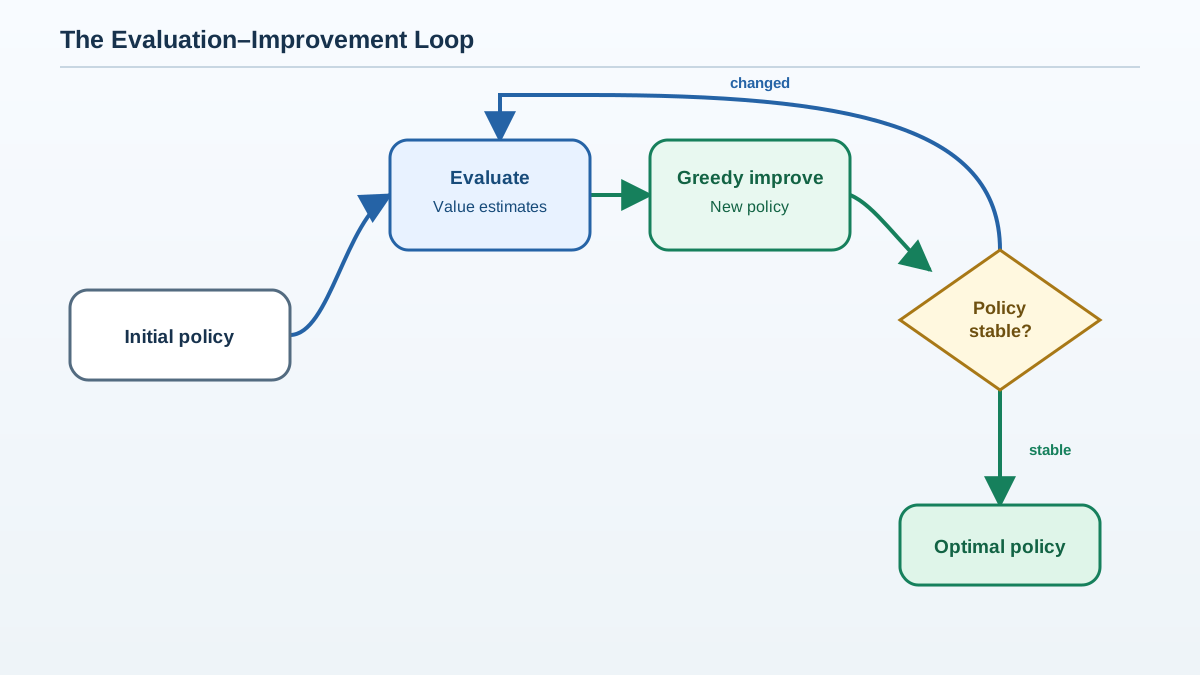
Policy iteration RL is the clean algorithm that resolves this problem by alternating the two steps until they stop changing.

The workflow is straightforward:

1. Start with an arbitrary policy, such as a random one.
2. Evaluate it fully: compute V^π for every state using iterative Bellman backups until the values converge.
3. Improve it greedily: for each state, compute Q^π(s, a) and set π(s) to the action with the highest value.
4. If the policy changed, go back to step 2. If it did not change, you have found the optimal policy.

For a finite MDP, this loop is guaranteed to converge to the optimal policy. Each improvement step produces a strictly better policy (or the same one, in which case you are done), and there are only finitely many policies, so the process cannot cycle forever.

The Geometric Picture

Sutton and Barto describe a useful mental image. Imagine a two-dimensional space where every point represents a combination of a value function and a policy. Draw two lines through this space:

• The value line contains points where the value function is accurate for the policy.
• The policy line contains points where the policy is greedy with respect to the value function.

Policy evaluation moves you toward the value line: it makes your value estimates match your current policy. Policy improvement moves you toward the policy line: it makes your policy greedy with respect to your current values.

Each step moves you closer to one line and further from the other. But together, the two processes push you toward the intersection of both lines—the point where the value function is accurate and the policy is greedy. That intersection is the optimal solution.

The Cost Problem

Full policy evaluation is expensive. Converging V^π for every state requires sweeping through the entire state space many times. For a small grid world, that is fine. For any realistic problem, it is not.

This is the tension that motivates everything that comes next. The clean algorithm works, but its cost profile is unacceptable for large problems. The solution is not to abandon the loop—it is to loosen it.

Generalized Policy Iteration: The Pattern Behind Most RL

Generalized policy iteration (GPI) is the observation that the two processes do not need to complete fully before alternating. They can interleave at any granularity.

Instead of evaluating the policy to convergence, you can run a few backup sweeps and then improve. Instead of improving every state at once, you can update a single state's action and then resume evaluation. The two processes chase each other, and as long as both keep making progress, the combination converges.

This is not a minor implementation detail. It is the reason almost every RL control method works.

Consider what happens with partial steps. Suppose your value estimates are somewhat inaccurate for the current policy. A greedy improvement based on those estimates might not produce a strictly better policy. But it will usually produce a different policy, and re-evaluating that policy will give you better value estimates, which will make the next improvement more reliable. The two processes correct each other's errors over time.

The geometric picture still applies, but the trajectory becomes messier. Instead of cleanly bouncing between the two lines, the point zigzags toward the intersection, sometimes overshooting, sometimes undershooting, but always making net progress.

GPI in Practice

Almost every RL control method is an instance of GPI:

• Q-learning interleaves a single backup (partial evaluation) with a greedy action selection (partial improvement) at every time step.
• SARSA does the same, but improves toward the action the policy actually takes rather than the greedy one.
• Actor-critic methods maintain two separate structures: the critic performs evaluation by estimating values, and the actor performs improvement by adjusting the policy in the direction of higher values.
• Deep RL methods like DQN or PPO are GPI with neural networks serving as function approximators for the value function, the policy, or both.

The pattern is the same everywhere. Evaluation and improvement push against each other until they reach consistency.

Tip: When you read about a new RL algorithm, the first question to ask is not "what is the loss function?" It is "where is the evaluation step, and where is the improvement step?" Once you can identify both, the algorithm stops being a black box.

Common Mistakes and How to Read Them

Here are the failure patterns I see most often when learners build their mental model of policy improvement.

Mistake 1: Treating a Single Greedy Step as a Finished Solution

Symptom: You evaluate a random policy, greedify it once, and report the result as "the optimal policy."

The problem: Improvement only matters relative to the policy being evaluated. Your value estimates described the random policy, not the greedy one. The greedy policy needs its own evaluation before you can trust the next improvement.

Corrected model: Improvement is a step in a loop, not a one-shot operation. The guarantee is about the process of alternating, not about any single greedy switch.

Mistake 2: Confusing Improvement from V with Improvement from Q

Symptom: You have a table of V values and try to pick actions by comparing state values directly.

The problem: State values do not tell you which action leads to which state. Comparing V(s₁) and V(s₂) does not tell you whether moving to s₁ is better than moving to s₂, because the actions available and their transition probabilities matter.

Corrected model: To improve from V, you need the environment model to compute Q. To improve directly from Q, you just compare action values. Know which quantity you have and what it requires.

Mistake 3: Expecting Value Estimates to Stay Valid After the Policy Changes

Symptom: You improve the policy and then use the old value estimates to make decisions, wondering why performance drops.

The problem: Value functions are policy-dependent. Change the policy, and the values change with it. The old estimates describe what would happen under the old policy, not the new one.

Corrected model: Every policy change invalidates your value estimates. Re-evaluation is not optional cleanup; it is a required step in the loop.

Mistake 4: Assuming GPI Guarantees Monotonic Improvement with Function Approximation

Symptom: You train a deep RL agent, see the policy get worse for a stretch, and conclude the algorithm is broken.

The problem: The clean convergence guarantees of policy iteration hold for tabular, finite MDPs with full evaluation. When you use neural networks to approximate values or policies, those guarantees weaken. The GPI pattern still guides intuition, but individual steps can make things worse before they get better.

Corrected model: GPI is a lens for understanding how RL methods work, not a guarantee of monotonic improvement in every setting. The theory tells you what is possible in the clean case; practice requires tolerating noise and approximation error.

When This Pattern Applies and When It Does Not

It helps to be precise about what is known, what is inferred, and what should not be assumed.

What is known: For tabular, finite MDPs with full or near-full policy evaluation, policy iteration converges to the optimal policy. The policy improvement theorem guarantees that each greedy step produces a policy at least as good as the previous one.

What is inferred: The GPI pattern—loose, interleaved alternation of evaluation and improvement—is a useful unifying lens for understanding most RL control methods. This is a conceptual framework, widely adopted in the field, not a formal theorem with universal guarantees.

What should not be assumed: That GPI guarantees monotonic improvement when function approximation is involved. Neural network policies and value functions can degrade temporarily, and the clean convergence story does not transfer automatically.

The practical takeaway is to use GPI as your mental map for reading any RL algorithm. Identify the evaluation process and the improvement process. Ask how completely each one runs before the other takes over. Ask what assumptions the method relaxes—partial evaluation, partial improvement, function approximation, or all three.

Your Next Step

The fastest way to make this concrete is to trace one full cycle by hand. Take a tiny tabular environment—a 3×3 grid with a goal state works well. Start with a random policy. Evaluate it fully using Bellman backups. Then improve it greedily. Then evaluate again. Watch how the value estimates change after the policy changes, and watch how the policy stabilizes after a few cycles.

Alternatively, take an algorithm you already know—Q-learning is a good candidate—and identify which part is the evaluation step and which part is the improvement step. In Q-learning, the update rule is partial evaluation, and the max over actions is partial improvement. Once you can see both processes inside a familiar algorithm, you will never read an RL method the same way again.

GPI is the reusable lens. Every control method you encounter from here on—value-based, policy-based, actor-critic, deep or tabular—is a variation on this single pattern: evaluate, improve, repeat.

References

Research updated Sep 9, 2026