Derive the Lagrangian and Primal-Dual Update for a Constrained MDP

You write down the problem cleanly: maximize expected reward, keep expected cost under a budget. Then you freeze, because there is no obvious place to put the constraint. You cannot subtract it from the reward without choosing a penalty weight by hand, and a hand-chosen weight is a guess that only sometimes lands on the budget you wanted.

The fix is to stop guessing the price of the constraint and let the optimization set it. That price is the Lagrange multiplier, and the machinery that updates it is a primal-dual loop. This article derives both from the constrained problem, then draws a hard line between the optimization construction and any claim about safety.

What the Constraint Actually Says

Before any multiplier appears, fix the problem. A constrained Markov decision process extends an ordinary MDP with a second signal. You have states $s \in \mathcal{S}$, actions $a \in \mathcal{A}$, a transition kernel $P(s' \mid s, a)$, and a discount factor $\gamma \in [0, 1)$. Alongside the reward $r(s, a)$, the environment emits a cost $c(s, a)$.

A policy $\pi$ induces two discounted value functions from a fixed initial-state distribution $\mu$:

$J(\pi) = \mathbb{E}_{\pi}\!\left[\sum_{t=0}^{\infty} \gamma^t\, r(s_t, a_t)\right], \qquad C(\pi) = \mathbb{E}_{\pi}\!\left[\sum_{t=0}^{\infty} \gamma^t\, c(s_t, a_t)\right].$

The constrained problem is:

$\max_{\pi} \; J(\pi) \quad \text{subject to} \quad C(\pi) \le d.$

Every symbol now has a referent. The constraint is an inequality on an expected discounted cost, evaluated from $\mu$, not a per-episode cap. That distinction will matter later.

If you have read the prerequisite concept article, you already have the penalty-versus-constraint distinction. The short version: a penalty discourages bad behavior, a constraint restricts the set of admissible policies. We do not re-derive that here. What we need is the machinery that turns the restriction into something an optimizer can actually run.

The derivation leans on three assumptions. State and action spaces are finite. At least one feasible policy exists, so the constraint set is nonempty. And the constraint is evaluated in expectation over $\mu$. Break any of these and the guarantees below weaken or vanish.

Why You Cannot Just Subtract the Constraint

The tempting move is to fold the cost into the reward: define $r'(s, a) = r(s, a) - \beta\, c(s, a)$ and run any standard RL algorithm. This works, in the narrow sense that it produces a policy. It fails as a way to hit a budget.

The penalty weight $\beta$ picks the reward-cost trade-off for you. You choose $\beta$, and the resulting policy satisfies $C(\pi) \le d$ only by accident. Run the same $\beta$ on a different seed or a slightly different environment and the realized cost drifts. There is no closed-form inverse that maps $\beta$ to a budget, because the constraint is a hard inequality on a quantity the agent only observes through sampling. You are tuning a dial whose units you cannot read.

The Lagrangian changes the question. Instead of asking "what penalty weight produces the budget?", it asks "what price makes the budget bind?" The optimization answers that, and the answer is a number you can inspect.

Warning: The Lagrangian is an optimization device. It reformulates the problem so a solver can attack it. It is not a safety mechanism, and it does not make the constraint unbreakable.

Building the Lagrangian Step by Step

Attach a multiplier $\lambda \ge 0$ to the cost-budget gap and write:

$\mathcal{L}(\pi, \lambda) = J(\pi) - \lambda\bigl(C(\pi) - d\bigr).$

Three pieces. The reward term $J(\pi)$ is what you want to grow. The priced violation term $-\lambda(C(\pi) - d)$ charges the policy when it overspends and credits it when it underspends. The constant $\lambda d$ is an offset that shifts the whole expression but does not change which policy is best for a fixed $\lambda$.

Now ask what the inner minimization over $\lambda \ge 0$ does. Two cases.

If $C(\pi) \le d$, the gap $C(\pi) - d$ is nonpositive. Multiplying by $\lambda \ge 0$ gives a nonpositive number, so $-\lambda(C(\pi) - d) \ge 0$. The inner minimum over $\lambda$ is attained at $\lambda = 0$, and $\mathcal{L}$ collapses to $J(\pi)$.

If $C(\pi) > d$, the gap is positive. As $\lambda \to \infty$, the term $-\lambda(C(\pi) - d) \to -\infty$. The inner minimum is unbounded below, so infeasible policies are driven to $-\infty$.

That is the whole trick. The inner minimization over $\lambda$ acts as a switch: feasible policies keep their reward, infeasible policies are annihilated. So

$\max_{\pi} \min_{\lambda \ge 0} \mathcal{L}(\pi, \lambda)$

recovers the constrained optimum. This max-min ordering is the primal problem.

The useful move is to swap the order. Under saddle-point conditions, the min and max commute:

$\max_{\pi} \min_{\lambda \ge 0} \mathcal{L}(\pi, \lambda) = \min_{\lambda \ge 0} \max_{\pi} \mathcal{L}(\pi, \lambda).$

The right-hand side is the dual problem, and it is the one that gives you an algorithm. The inner $\max_\pi$ is an ordinary unconstrained MDP for any fixed $\lambda$. The outer $\min_\lambda$ is a one-dimensional search over a price.

Reading the Multiplier as a Price

$\lambda$ is the marginal cost of tightening the budget by one unit. Economists call this the shadow price of the constraint, and the name earns its keep here.

When $\lambda = 0$, the constraint is slack. The unconstrained reward-maximizing policy already respects the budget, so the price of the constraint is zero. When $\lambda$ is large, the constraint binds hard and the agent trades reward for feasibility. The multiplier is not a hyperparameter you tune. It is a quantity the optimization discovers.

The mechanism becomes concrete when you look at the inner problem. For a fixed $\lambda$,

$\max_{\pi} \; J(\pi) - \lambda\, C(\pi) = \max_{\pi} \; \mathbb{E}_{\pi}\!\left[\sum_{t=0}^{\infty} \gamma^t \bigl(r(s_t, a_t) - \lambda\, c(s_t, a_t)\bigr)\right].$

That is an ordinary MDP with modified reward $r(s, a) - \lambda\, c(s, a)$. Any standard RL algorithm can solve it. The constrained problem has been reduced to a sequence of unconstrained ones, each indexed by a price.

A Two-Policy Toy

Take a CMDP with two candidate policies and $d = 1.0$.

$\pi_A$ is infeasible ($3.0 > 1.0$). $\pi_B$ is feasible. For a fixed $\lambda$, the Lagrangian values are:

$\mathcal{L}(\pi_A, \lambda) = 10 - \lambda(3.0 - 1.0) = 10 - 2\lambda, \qquad \mathcal{L}(\pi_B, \lambda) = 7 - \lambda(0.5 - 1.0) = 7 + 0.5\lambda.$

Set them equal: $10 - 2\lambda = 7 + 0.5\lambda$, so $\lambda = 1.2$. Below $\lambda = 1.2$, the infeasible policy wins because its reward advantage outweighs the price. Above it, the feasible policy wins. The multiplier is exactly the price at which the agent becomes indifferent between breaking the budget and respecting it.

Deriving the Primal-Dual Update

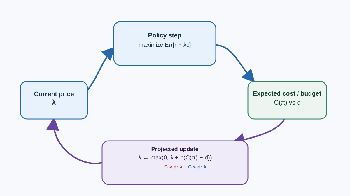
The dual problem is $\min_{\lambda \ge 0} \max_{\pi} \mathcal{L}(\pi, \lambda)$. We attack it by alternating: fix one variable, improve the other.

Primal step. Fix $\lambda$. Ascend the gradient of $\mathcal{L}$ with respect to the policy parameters $\theta$. Since $\lambda$ is constant, this is gradient ascent on the modified reward $r(s, a) - \lambda\, c(s, a)$. For a tabular or softmax policy, that is an ordinary policy-gradient step.

Dual step. Differentiate $\mathcal{L}$ with respect to $\lambda$:

$\frac{\partial \mathcal{L}}{\partial \lambda} = -\bigl(C(\pi) - d\bigr) = d - C(\pi).$

This derivative is negative exactly when the constraint is violated ($C(\pi) > d$) and positive when it is satisfied. The outer problem is a minimization over $\lambda$, so we descend this derivative. Descending $d - C(\pi)$ means stepping in the direction that increases $C(\pi) - d$ when the constraint is violated. Written as an ascent on the violation:

$\lambda \leftarrow \lambda + \eta\, \bigl(C(\pi) - d\bigr).$

When cost exceeds the budget, $\lambda$ rises and the modified reward penalizes cost harder. When cost sits below the budget, $\lambda$ falls and the agent is free to chase reward again.

Projection. The derivation assumed $\lambda \ge 0$. The raw update can push $\lambda$ negative when the constraint is comfortably satisfied. So project after every step:

$\lambda \leftarrow \max\bigl(0, \; \lambda + \eta\, (C(\pi) - d)\bigr).$

The projection is what enforces the nonnegativity the math required. Without it, a negative multiplier would reward cost rather than penalize it, and the whole construction inverts.

Note: The two updates run on different timescales. The primal chases the best policy for the current price; the dual chases the price that makes the budget bind. In practice the dual usually steps more slowly, so the primal has time to adapt before the price moves again.

Continuing the Toy

Start at $\lambda_0 = 0$, $\eta = 0.5$. At $\lambda = 0$, $\pi_A$ wins with $\mathcal{L} = 10$, and $C(\pi_A) = 3.0$.

Watch the mechanism. While the constraint is violated, $\lambda$ climbs. Once the price crosses $1.2$ and the feasible policy takes over, cost drops below the budget and $\lambda$ eases back. The multiplier oscillates around the indifference point, and the cost oscillates around the budget. That is the primal-dual loop doing its job.

What the Derivation Does Not Promise

This is the part most treatments skip, and it is the part that keeps you out of trouble.

The Lagrangian reformulation is exact only under convexity and saddle-point conditions. Policy parameterization makes the primal problem non-concave in general, so the min-max swap is not guaranteed to hold. Convergence is a property of specific algorithms under specific assumptions, not a property of the derivation itself.

Feasibility is not guaranteed. If no policy satisfies the budget, the dual diverges and there is nothing to converge to. The method cannot manufacture a feasible policy out of an infeasible problem.

Expected-cost constraints are satisfied in expectation over $\mu$. A single episode can still blow through the budget badly. If your cost is catastrophic in one trajectory, an expectation is the wrong object to constrain.

Multiplier oscillation and slow dual convergence are common. $\lambda$ is a learned quantity with its own stability problems, and it can wander for a long time before settling.

Common mistake: Treating a converged $\lambda$ as proof that the policy is safe. It is proof that the expected cost landed near the budget on the runs you measured. Those are different claims.

The decision rule: use this when you want a tunable reward-cost trade-off with a principled price. Do not use it as a substitute for action masking, shielding, or hard runtime limits. Those enforce; the Lagrangian negotiates.

Where to Take This Next

The smallest useful test is a tabular primal-dual loop on a toy CMDP. Implement the two updates above, log $\lambda$ and the realized cost each iteration, and plot cost against the budget over time. You will see the oscillation from the toy example appear in your own numbers.

Watch for two failure signatures. If $\lambda$ climbs without cost dropping, your policy may be unable to reach feasibility, or your dual step size is too large. If cost drops below budget while reward collapses, $\lambda$ is overshooting and the agent is paying too much for a constraint that was already satisfied.

The durable rule: the multiplier is a price, the projection is the guardrail, and neither one is a safety guarantee. When you are ready to see the fixed-penalty baseline and the primal-dual method run side by side on the same toy problem, that comparison is where the theory meets measured cost.