
Compare Mean Return and Downside-Sensitive Policy Choices in a Toy Task
Two policies. One wins on average. The other wins on the days you actually have to survive. If your selection rule can't tell them apart, you're not…

Key topics
Two policies. One wins on average. The other wins on the days you actually have to survive. If your selection rule can't tell them apart, you're not choosing a policy — you're choosing a coin flip and calling it a decision.
This exercise makes that distinction concrete. You'll define three fixed policies as return distributions, sample episodes from each, rank them by mean return, then rank them again by a downside-sensitive criterion. The goal is to watch the ranking flip and understand exactly which samples caused it.
What This Exercise Builds and What You Need
The task is narrow by design: three frozen policies, sampled returns, two ranking criteria. No learning, no Bellman updates, no environment dynamics. The selection criterion is the only variable.
That constraint matters. If you tune the policies after seeing the results, you haven't tested a criterion — you've tested your own search. Frozen parameters keep the comparison honest.
Dependencies: Python 3, NumPy, and optionally Matplotlib for a histogram. No RL library, no GPU, no credentials.
Assumed context: You already know that a return is a random variable, not a score, and that a policy induces a distribution over returns. If that's shaky, the short version is: the same policy run on the same task produces different outcomes because the environment and the policy both have randomness baked in. We're working with those distributions directly.
Success criterion: The two rankings disagree, and you can point to the specific samples that caused the disagreement.
Design Three Policies With Deliberately Different Tails
We need distributions whose means and lower tails conflict. Here's the parameter table:
| Policy | Description | Mean | Left tail |
|---|---|---|---|
| A | Usually pays well, occasionally fails badly | High | Heavy |
| B | Modest but consistent | Lower | Tight |
| C | Middle case | Medium | Moderate |
Policy C exists to keep the comparison honest. Without it, you could reduce the lesson to "safe beats greedy," which misses the point.
import numpy as np

def sample_policy_a(rng, n):
    # 90% of episodes: return around +10
    # 10% of episodes: return around -50
    base = rng.normal(10, 2, n)
    tail_mask = rng.random(n) < 0.10
    base[tail_mask] = rng.normal(-50, 5, tail_mask.sum())
    return base

def sample_policy_b(rng, n):
    # Tight distribution around +5
    return rng.normal(5, 1.5, n)

def sample_policy_c(rng, n):
    # 85% around +8, 15% around -20
    base = rng.normal(8, 2, n)
    tail_mask = rng.random(n) < 0.15
    base[tail_mask] = rng.normal(-20, 4, tail_mask.sum())
    return base
A quick sanity check before moving on: plot the three distributions on one axis with the mean marked on each. You should see Policy A's mean sitting to the right of Policy B's, but with a long shadow stretching left.
Knowledge check
Check your understanding
Answer this question before you continue.
Sample Episodes and Compute Mean Return
Draw N episodes per policy from the same seeded generator. The shared seed makes the run reproducible — rerun it and you get the same numbers. It does not pair the policies, because each sampler consumes the random stream differently. Reproducibility is the goal here, not matched episode conditions.
def run_comparison(n_episodes=10000, seed=42):
    rng = np.random.default_rng(seed)
    policies = {
        "A": sample_policy_a,
        "B": sample_policy_b,
        "C": sample_policy_c,
    }
    returns = {name: fn(rng, n_episodes) for name, fn in policies.items()}
    return returns

returns = run_comparison()
for name, r in returns.items():
    print(f"Policy {name}: mean = {r.mean():.2f}")
Expected output shape:
Policy A: mean = 4.02
Policy B: mean = 5.01
Policy C: mean = 3.78
Policy B wins on mean. That's the setup — and it's the part that surprises people. Policy A looks like the aggressive, high-reward choice, but its 10% failure rate drags the average below the modest, consistent policy.
Common mistake: Using a different seed per policy and then comparing the numbers as if they were the same experiment. One generator, one seed, all policies — so that when you rerun, you're rerunning the same experiment.
The sample mean is an estimate. With finite N, the ranking itself is noisy. Increase N and confirm the mean ranking stabilizes — if it doesn't, your sampler or seed handling is wrong.
Knowledge check
Check your understanding
Answer this question before you continue.
Add One Downside-Sensitive Criterion
We'll use CVaR (Conditional Value at Risk) at a fixed confidence level. In plain terms: the average of the worst alpha-fraction of returns. If alpha is 0.10, CVaR is the mean of the bottom 10% of episodes.
Why CVaR and not variance? Variance punishes upside and downside equally. That's the wrong shape for a downside question. A policy that occasionally returns +200 is not "risky" in the way we care about here. This is a deliberate choice, not a claim that CVaR is universally better.
def cvar(returns, alpha=0.10):
    sorted_r = np.sort(returns)
    n_tail = int(np.ceil(len(sorted_r) * alpha))
    return sorted_r[:n_tail].mean()
The boundary condition: when N * alpha isn't an integer, we round up. Pick a convention, state it, and keep it consistent. Rounding up means the tail always contains at least one sample.
Sign convention: A higher (less negative) CVaR means a better-protected lower tail. Policy B's CVaR will be around +2 or +3. Policy A's will be deeply negative. Get this backwards and every conclusion inverts.
Warning: Sign errors here are the most common silent bug. Print the tail samples alongside the CVaR value the first time you run it.
Knowledge check
Check your understanding
Answer this question before you continue.
Compare the Two Rankings and Read the Disagreement
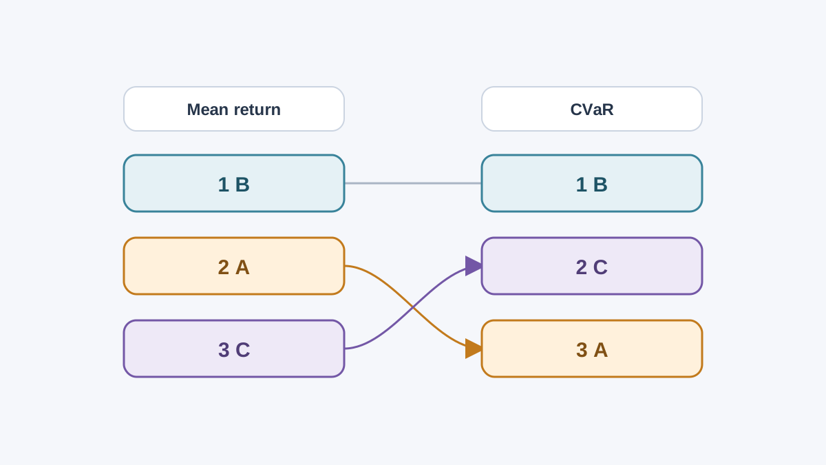
print(f"{'Policy':<8} {'Mean':>8} {'CVaR':>8} {'Rank(Mean)':>12} {'Rank(CVaR)':>12}")
means = {n: r.mean() for n, r in returns.items()}
cvars = {n: cvar(r) for n, r in returns.items()}
mean_rank = sorted(means, key=means.get, reverse=True)
cvar_rank = sorted(cvars, key=cvars.get, reverse=True)
for name in ["A", "B", "C"]:
    print(f"{name:<8} {means[name]:>8.2f} {cvars[name]:>8.2f} "
          f"{mean_rank.index(name)+1:>12} {cvar_rank.index(name)+1:>12}")
Expected result: Policy B wins on mean and loses on CVaR. Policy A does the reverse. Policy C lands somewhere in between.
The mechanism is straightforward. The mean is sensitive to the whole distribution but dominated by the bulk — those 90% of episodes returning +10 pull it up. CVaR ignores everything above the tail threshold. Different questions, different answers.
| Criterion | Rewards | Ignores | Misleading when |
|---|---|---|---|
| Mean return | Bulk performance | Tail severity | A single bad episode is unrecoverable |
| CVaR | Tail protection | Upside | Tail estimate rests on few samples |
Decision boundary: Mean return is the right criterion when the downside is recoverable and repeated. A downside criterion earns its place when a single bad episode is unrecoverable, or when the tail outcome is the one you actually have to survive.
When not to use a downside criterion: if the tail estimate rests on a handful of samples, CVaR is mostly noise. Check how many samples land in the tail before trusting the number.
Knowledge check
Check your understanding
Answer this question before you continue.
Break It on Purpose: Three Failure Modes to Reproduce
A criterion you've never seen break is a criterion you don't yet understand. Trigger these deliberately.
Too few samples. Shrink N to 200. Rerun with different seeds. Watch the CVaR ranking flip. The signal: a ranking that changes on rerun. The fix: increase N until the ranking stabilizes across seeds.
Tail too thin. Set alpha to 0.001 with N=1000. Now one sample defines CVaR. Observe how a single episode controls the policy choice. The fix: keep the tail count in the dozens at minimum.
Seed sensitivity. Rerun the whole comparison with several different seeds and record how often the CVaR ranking holds. The signal: a ranking that flips across seeds means your sample size is too small for the confidence level you chose. The fix: raise N, raise alpha, or both — then confirm the ranking is stable before you trust it.
Tip: Frame these as evidence, not embarrassment. Every one of them is a real failure mode you'll encounter when comparing policies on actual agents.
One Modification Worth Trying Next
Sweep alpha across a small range — 0.01, 0.05, 0.10, 0.25 — and plot how the CVaR ranking changes. Some policies only look safe at one confidence level. Policy C might beat Policy B at alpha=0.25 but lose at alpha=0.05, because its tail is thinner but deeper.
Or add a fourth policy that's a near-copy of A with a slightly heavier tail, and find the point where the ranking flips. Report what you changed, what you expected, and what the output actually showed. That habit is the whole point.
The criterion you optimize is a decision about which failures you're willing to accept — not a neutral measurement. Rerun this comparison with your own policy parameters, or carry the same mean-versus-tail check into the next experiment you design. The natural follow-on is choosing an objective for an agent that actually learns, rather than a frozen policy you've already defined.
Knowledge check
Final check
Finish the article by checking the ideas you just learned.
References
Build a stronger RL mental model
Use structured resources to connect equations, algorithms, and observable agent behavior.


