
CVaR Objectives for Risk-Sensitive Reinforcement Learning
Two policies. Same expected return. One of them occasionally produces an episode so bad you would never deploy it. The mean cannot tell them apart — not…

Key topics
Two policies. Same expected return. One of them occasionally produces an episode so bad you would never deploy it. The mean cannot tell them apart — not because it is poorly estimated, but because it was never built to see the difference.
That is the gap CVaR fills. Conditional Value-at-Risk asks a narrower, sharper question than expected return: among my worst outcomes, how bad are they on average? This article defines that criterion, computes it by hand on a small distribution, proves with a paired example that it can flip a policy ranking, places it next to mean-return optimization and cost constraints, and then states where the interpretation quietly breaks.
Why the Mean Hides the Tail
You already know returns are random variables with distributions, and that risk preference is a separate axis from uncertainty. The consequence is blunt: a policy that earns 10 on average by winning big and losing catastrophically can be indistinguishable, in expectation, from a policy that earns 10 by grinding out steady results.
The mean is a single number summarizing an entire distribution. It is blind to shape by construction. When the downside is merely unpleasant, that blindness is fine — you want the highest average and you accept the variance. When the downside is unacceptable, the mean is answering a question you did not ask.
The decision the mean cannot make is the one where you must choose between a steady policy and a high-variance policy whose bad tail you cannot tolerate. Downside risk in reinforcement learning is exactly this problem: you need a criterion that reads the shape of the distribution, not just its center.
Notation: Returns, Quantiles, and the Risk Level
Fix the symbols before any formula appears, because sign conventions are the single most common source of confusion here.
Let be the return of a fixed policy — a random variable, with the convention that higher is better. This matters immediately: CVaR is often written in finance for losses, where lower is better. A criterion written for losses is the negation of one written for returns. Mix them silently and you invert your policy preference.
Let be the risk level: the fraction of worst outcomes you are willing to reason about. Small means you care about a thin, deep tail. Large means you care about a broad slice of bad outcomes.
Define the quantile — the cutoff that separates the worst fraction of outcomes from the rest. That cutoff value is the Value-at-Risk, .
VaR names a threshold. It says nothing about how far past the threshold outcomes fall. A policy whose worst 5% all land just below the cutoff and a policy whose worst 5% fall off a cliff have the same VaR. That limitation is precisely what CVaR repairs.
Note: Think of VaR as the fence and CVaR as the average depth of everything on the wrong side of it. A fence tells you where the boundary is. It does not tell you how bad the fall is.
Knowledge check
Check your understanding
Answer this question before you continue.
Defining CVaR as an Average of the Worst Cases
In plain language: CVaR is the average return among the worst fraction of outcomes. Not the cutoff — the average of what lies beyond it.
For a continuous distribution, the conditional-expectation form is exact:
Read it as: condition on being in the tail, then average. For discrete distributions this needs care, because the tail boundary may cut through a probability atom. We will handle that case directly in the worked example.
The form that makes CVaR usable in optimization is the variational representation:
where . This looks heavier than it is. The variable is a candidate threshold. The term measures how far outcomes fall below that threshold, on average. Maximizing over finds the threshold that best balances the cutoff against the scaled shortfall — and the value at that optimum is the tail average. The optimizer is the VaR.
Why does this form matter? It is convex and differentiable enough for gradient-based optimization, which is why CVaR shows up in policy-gradient work rather than staying a descriptive statistic.
Two endpoints anchor the intuition:
- recovers the ordinary expected return. You are averaging over the entire distribution.
- drives the criterion toward the worst-case outcome — the essential infimum of the return.
CVaR is also a coherent risk measure: it satisfies monotonicity and subadditivity, meaning the risk of a combined position never exceeds the sum of the parts. The quantile alone does not have this property. Coherence is what makes CVaR behave sensibly when you combine risks rather than treating each in isolation.
Knowledge check
Check your understanding
Answer this question before you continue.
Worked Example: CVaR on a Small Discrete Return Distribution
Take a policy with four possible returns and explicit probabilities:
| Return | Probability |
|---|---|
| 10 | 0.50 |
| 4 | 0.30 |
| 0 | 0.15 |
| −20 | 0.05 |
Expected return. Sum the products: .
Now compute CVaR at — the average of the worst 10% of outcomes.
Step 1: find the quantile. Accumulate probability from the bottom. The worst outcome, , carries probability 0.05. That is less than 0.10, so the cutoff is not at . Adding the next outcome, , brings cumulative probability to , which crosses 0.10. So the -th quantile is .
Step 2: handle the atom. The tail we want has total probability 0.10. The outcome contributes 0.05 of it. The remaining 0.05 must come from the boundary outcome — but only partially, since carries 0.15 of probability and we only need a third of it.
Step 3: average the tail.
The tail average is . The plain expected return is . The gap — points — is the cost of the tail the mean was hiding. A policy scored at on average is, in its worst decile, losing per episode.
Common mistake: Averaging only the outcomes strictly below the quantile. When cuts through an atom, you must weight the boundary outcome by exactly the probability needed to reach . The variational form handles this automatically; hand arithmetic does not unless you are careful.
Knowledge check
Check your understanding
Answer this question before you continue.
When CVaR Changes the Decision
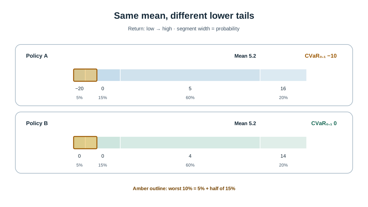
A single distribution shows that the tail differs from the mean. It does not yet show that CVaR changes a choice. For that, you need two policies with the same mean and different tails.
Call the first policy — the one above. Now consider policy :
| Return | Probability |
|---|---|
| 8 | 0.50 |
| 4 | 0.30 |
| 2 | 0.15 |
| −2 | 0.05 |
Expected return of : .
That is not a tie. Adjust the top outcome to : . Now both policies have mean .
CVaR of at . The worst outcome is with probability 0.05. The next outcome is with probability 0.15, so cumulative probability crosses 0.10 at . The tail needs 0.10 total; supplies 0.05, and supplies the remaining 0.05.
Now compare:
| Policy | Mean return | CVaR at |
|---|---|---|
| 5.2 | −10 | |
| 5.2 | 0 |
The means are identical. The tail averages are ten points apart. Under mean optimization, and are interchangeable. Under CVaR at , wins decisively — its worst decile averages zero, while 's worst decile averages a loss of ten per episode.
This is the whole argument in one table. The mean is not wrong; it is answering a different question. CVaR reads the shape the mean cannot see, and that shape can flip the ranking.
CVaR Versus Mean Return and Cost Constraints
These three objectives are neighbors, not synonyms. Choosing the wrong one is a modeling error, not a tuning error.
| Objective | What it optimizes | What it guarantees | Failure it does not prevent |
|---|---|---|---|
| Mean return | Expected value over all outcomes | Highest average | Catastrophic tail outcomes |
| CVaR | Average of the worst fraction | Better tail behavior at chosen | Violation of a hard feasibility boundary |
| Cost constraint | Reward subject to expected cost budget | The stated expected-cost budget, not per-episode safety | Poor tail shape inside the feasible set |
Against mean return. Mean optimization is the special case . CVaR does not merely rescore policies — it changes which policy is optimal, as the paired example just showed.
Against constrained formulations. A cost constraint enforces feasibility on an expected cost budget. CVaR reshapes the objective itself around the tail. They answer different questions and can disagree about the same policy: a policy can satisfy the expected-cost budget while still having a terrible tail, or have an acceptable tail while violating the budget. And satisfying an expected-cost constraint does not rule out individual catastrophic episodes — it targets an aggregate, not a per-episode boundary.
There is also a robust-MDP reading worth knowing. Optimizing CVaR of return has been characterized as optimizing expected value under a worst-case perturbation of the transition kernel. That equivalence explains why CVaR appeals in safety-critical settings — it is not just a preference, it is a form of robustness.
Decision rule. Pick CVaR when the harm is concentrated in rare outcomes and you can tolerate a lower average. Pick a constraint when the requirement is a hard feasibility boundary rather than a preference. If you need both, you need both — they compose, but neither substitutes for the other.
Knowledge check
Check your understanding
Answer this question before you continue.
Assumptions and Interpretation Caveats
The criterion is precise. The interpretation is where people go wrong.
The risk level is a modeling choice, not a discovered quantity. Different values select different policies. There is no neutral default. Choosing after seeing results is not choosing a criterion; it is choosing an outcome.
CVaR is defined on the return distribution of a fixed policy. Estimating it from a small number of sampled episodes is noisy — the tail is by definition the part of the distribution you observe least. Smaller requires more trajectories to estimate reliably, because the sample cost grows as the tail gets thinner.
Static and dynamic interpretations differ. The tail of the return distribution is not the same object as a per-step or time-consistent risk criterion. Naive action selection on distributional value estimates can converge to neither the dynamic, Markovian CVaR nor the static, non-Markovian CVaR. If you are building on distributional methods, this distinction is load-bearing.
Sign and normalization conventions vary across sources. A criterion written for losses is the negation of one written for returns. Mixing them silently inverts your policy preference.
What CVaR is not. It is not a safety guarantee. It is not a substitute for a feasibility constraint. It is not a fix for a misspecified reward — if your reward function is wrong, CVaR will optimize the wrong thing, just more carefully.
Where This Leaves You
One sentence to keep: CVaR is the average of your worst fraction of outcomes, and it is a preference over distributions, not a constraint on them.
The practical next move is small and concrete. Take two policies from an experiment you have already run. Compute CVaR at two or three risk levels by hand, using the atom-weighting step from the worked example. Then check whether the ranking flips. If it does, the mean was hiding a decision you needed to make.
That raises the evaluation question this criterion forces: how many episodes do you need before a tail estimate is stable enough to trust? That is the next thing to measure.
And the builder's rule that outranks all of it: choose the criterion before you run the comparison. A criterion chosen after seeing the results is not a criterion.
Knowledge check
Final check
Finish the article by checking the ideas you just learned.
References
Build a stronger RL mental model
Use structured resources to connect equations, algorithms, and observable agent behavior.


