Distributional Reinforcement Learning Explained: Predicting Return Distributions Instead of Averages

Two actions can offer the same expected return and still feel completely different to the agent that takes them. One delivers a steady, predictable outcome. The other is a coin flip between a windfall and a wipeout. A standard value function cannot tell them apart. Distributional reinforcement learning can—because it predicts the whole range of possible outcomes, not just the average.

What a Single Number Hides

If you have worked with value functions, you already know the core object: Q(s, a) estimates the expected return from taking action a in state s, then following the policy afterward. The word expected is doing a lot of work there. It compresses every possible future into one scalar.

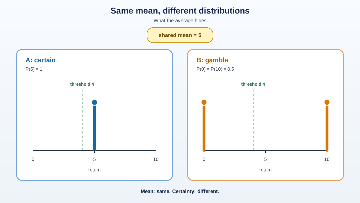
Consider a concrete choice. Action A guarantees a reward of 5. Action B gives you 10 with probability 0.5 and 0 with probability 0.5. Both have an expected value of 5. A Q-learning agent treats them as identical—same Q-value, same ranking, same greedy choice. But they are not the same experience. One is certain; the other is a gamble. If the agent needs a minimum return of 4 to survive until the next episode, Action A is safe and Action B fails half the time.

The mean is a summary, not the story. It tells you the center of the outcome distribution but discards its shape: the variance, the tails, the peaks, the possibility of catastrophe. Distributional reinforcement learning keeps the story by predicting the full distribution of returns instead of collapsing it into an expectation.

The Return Is a Random Variable, Not a Number

The shift starts with a reframing. In standard RL, the return is a number you estimate. In distributional RL, the return is a random variable—call it Z(s, a)—and the familiar Q-value is its expectation:

Q(s, a) = E[Z(s, a)]

That single equation contains the whole conceptual move. The value function you already know is one statistic of a richer object. Distributional RL predicts the object itself.

Where does the randomness in Z come from? Three sources, and it is worth naming all of them:

• Stochastic rewards. The environment may not return a fixed reward for a state-action pair. A slot machine pays out varying amounts; a trading environment produces variable profits.
• Stochastic transitions. The next state may not be deterministic. The same action in the same state can lead to different outcomes.
• A stochastic policy. Even in a deterministic environment, an exploring agent that sometimes takes random actions generates a spread of possible trajectories.

That last point surprises people. You can have a fully deterministic environment and still observe a distribution of returns, simply because the agent's own exploration injects randomness into which states it visits. The distribution is not just environmental noise; it is the compound result of everything uncertain between the current moment and the end of the episode.

Picture a single state-action pair as the root of a tree. Each branch is a possible next state, each branch after that another transition, and so on until the episode ends. The leaves of that tree are the possible returns. A value function averages the leaves. Distributional RL builds a histogram of them.

The Distributional Bellman Equation

The Bellman equation you already know relates expectations across time steps. The distributional version relates entire distributions. For a fixed policy π, the return distribution satisfies:

Z(s, a) = R(s, a) + γZ(s′, a′)

The equals sign here means "equal in distribution," not "equal as numbers." The sum is a sum of random variables, which means the distribution of Z(s, a) is built by combining three sources of randomness: the reward R, the next state-action pair (s′, a′), and the return distribution at that next pair.

This is the distributional Bellman equation, and it is the direct generalization of the scalar Bellman relationship you have seen in decision-tree form. The scalar version says the expected return now equals the expected reward plus the discounted expected return next step. The distributional version says the whole distribution of returns now equals the distribution of the reward plus the discounted return distribution next step.

The distributional Bellman operator composes those three sources of randomness into a new distribution. You can visualize it as a pipeline:

1. Take the next state-action return distribution.
2. Discount it—multiplying by γ shrinks the distribution toward zero, compressing its spread.
3. Shift it by the reward distribution.
4. Project the result back onto whatever representation you are using.

The scalar Bellman operator does the same dance with single numbers. The distributional operator does it with shapes. That is the entire difference, and it is also why the distributional version is harder: you cannot just add two numbers and store the result. You have to combine two probability distributions and keep the result representable.

Why the Mean Is Not Enough for Decisions

If the greedy policy only cares about expected value, why bother with the distribution? Because the distribution changes decisions in ways the mean cannot express.

Risk-sensitive objectives. An agent with a survival constraint—a minimum return threshold it must meet—should prefer the action with lower variance, even at the cost of a lower mean. A robot that needs to reach a charging station with enough battery remaining cares about the tail of the outcome distribution, not just its center. The mean alone cannot represent that preference.

Multimodal returns. Some distributions have two distinct peaks: a likely moderate outcome and a rare but large jackpot. The mean sits between the peaks, in a region of outcome space that may never actually occur. A policy optimized against that mean is optimizing for a future that does not exist. The distribution reveals the bimodal reality; the scalar hides it behind a misleading middle.

Exploration signal. High-variance outcomes are information. If an action produces wildly different returns depending on the state that follows, that variability signals uncertainty worth probing. A distributional agent can use the spread of predicted outcomes to guide where it explores next, rather than treating all actions with similar means as equally well understood.

None of this changes the greedy policy rule: when you must pick one action, you still maximize expected value. But the distribution informs the confidence you place in that expectation, the risk you are accepting, and whether the state deserves further investigation. The mean tells you what to do. The distribution tells you how much to trust that answer.

When does the mean suffice? In genuinely risk-neutral settings where only the long-run average matters and the variance is irrelevant. If you are averaging over many repeated decisions and have no survival threshold, the spread of outcomes washes out. The scalar value function is the right tool for that job.

How Distributional RL Is Represented in Practice

Predicting a full distribution requires choosing how to represent it. The main approaches each make a different tradeoff between expressiveness, stability, and computational cost.

Categorical approach (C51). Fix a set of support points—atoms—spread across a range of possible returns. The agent learns a probability for each atom, effectively building a histogram. The distributional Bellman target is projected onto these fixed atoms before the update. This was the approach in the paper that launched distributional RL as a practical method, and it is simple to understand: a fixed grid of buckets, with learned probabilities for each.

Quantile approach (QR-DQN). Instead of fixing the support and learning probabilities, fix the probabilities and learn the support. The distribution is represented as a uniform mixture of point masses at learnable quantile locations. This is more flexible than a fixed grid because the quantiles can spread or concentrate wherever the return distribution actually lives.

Implicit quantile networks (IQN). Go one step further: sample quantiles on demand rather than committing to a fixed set. The network takes a state, an action, and a sampled quantile level, and returns the corresponding return value. This makes the representation arbitrarily fine-grained at inference time.

All three share the same conceptual shift. They predict a distribution, not a scalar. The differences are engineering choices about how to parameterize that distribution and which loss function to minimize when comparing predicted and target distributions.

When Distributional RL Helps and When It Is Overkill

Distributional RL is not a free upgrade. It costs more computation, more representational complexity, and more careful engineering. Here is the decision boundary I use.

Use it when outcome variability changes your action choice. Stochastic rewards, risk-sensitive objectives, survival constraints, or any setting where the spread of outcomes matters for policy selection. If two actions have similar means but different risk profiles, and you care about the difference, you need the distribution.

Use it as a regularizer. Here is the surprising result: distributional methods often improve performance even when the distribution itself is never used for decisions. The richer prediction target seems to stabilize learning and produce better features, almost as a side effect. If you are already using a deep value-based agent and want a practical boost, distributional RL is worth trying even when you only read out the mean at decision time.

Skip it in deterministic environments. If the return distribution collapses to a single point, you are doing extra work to predict a number you already knew. The distribution adds nothing.

Skip it for genuinely risk-neutral problems. When only the long-run average matters and you have no constraints on individual outcomes, the scalar value function is sufficient and cheaper.

My practical rule: predict the full return distribution when outcome variability can change your action choice, or when the richer target stabilizes learning in a way you can measure. Fall back to a scalar value function when the environment is deterministic or the objective is genuinely risk-neutral.

The cleanest way to build intuition is to run a small experiment. Take a stochastic environment with two actions that share an expected return but differ in variance. Train one agent with Q-learning and one with a distributional method. Watch how they behave. The scalar agent will treat the actions as interchangeable. The distributional agent will show a clear preference the moment you add any risk sensitivity to its decision rule. That difference, visible in a few minutes of training, is the entire argument for distributional reinforcement learning in one observation.

References

Research updated Sep 9, 2026