Risk-Sensitive Reinforcement Learning: Choosing Policies Beyond Average Return

Two policies can share the exact same expected return and still feel completely different to the person who has to live with the outcomes. One delivers steady, predictable performance run after run. The other produces good results most of the time but occasionally collapses into a catastrophic episode the operator cannot absorb. Maximize expected return and the optimizer literally cannot tell them apart.

That blindness is not a bug in your implementation. It is a property of the objective itself.

Why Average Return Can Pick the Wrong Policy

Expected return is one statistic of a return distribution. It tells you where the center sits, and nothing else. Spread, skew, tail weight, the probability of ruin—all of it is invisible to an objective that only averages.

Consider a concrete scenario. Policy A returns 100 in every episode. Policy B returns 110 in 90% of episodes and −80 in the remaining 10%. Both have an expected return of 100. If you are running a system where a single −80 outcome means a crashed vehicle, a rejected batch, or a regulatory violation, the mean-optimal choice is not merely suboptimal. It is unacceptable.

Risk-neutral reinforcement learning is only the right objective when the operator can absorb every outcome equally. That condition is rarely true in deployment. A trading desk can tolerate a bad quarter. An autonomous vehicle cannot tolerate a bad intersection. The same environment, the same reward function, and the same mean can hide two entirely different operational realities.

Choosing to go risk-sensitive is a statement about the operator's downside tolerance. It is not a property of the environment. The environment has a return distribution; the objective selects which part of that distribution the agent optimizes. Expected return is one legitimate choice among many, and treating it as the default is itself a risk preference—one that says "I do not care how the outcomes are spread."

This builds directly on the return-distribution view from distributional RL. Once you stop collapsing outcomes into a single number and start thinking about the full distribution of possible returns, the question is no longer "what is the best policy?" but "what part of this distribution am I willing to ignore?"

Separating Risk, Uncertainty, and Safety

Before choosing a risk-sensitive objective, you need to be precise about which problem you are actually solving. Three concepts get conflated constantly, and each routes you to a different tool.

Aleatoric risk is the inherent randomness in the environment itself. Transitions and rewards have stochastic structure, and no amount of data will remove it. A slot machine has aleatoric risk. So does a trading environment, a robotic manipulation task with sensor noise, or a driving scenario with unpredictable other agents.

Epistemic uncertainty is the agent's ignorance about the environment. It shrinks as the agent collects more data. A new environment with unknown transition probabilities carries epistemic uncertainty; the same environment after ten thousand episodes carries much less.

Safety constraints are hard limits on behavior. Certain actions, states, or outcomes are simply not allowed, regardless of their expected value.

Risk-sensitive objectives target aleatoric variability in the return. They reshape what the agent optimizes. Epistemic uncertainty is the domain of exploration bonuses and regret analysis—you reduce it by gathering information, not by changing the objective. Safety constraints are the domain of constrained RL: you forbid what the agent may do, rather than tilting what it prefers.

A risk measure changes what the agent optimizes. A constraint changes what the agent is allowed to do. These are different levers, and pulling the wrong one produces a policy that either ignores the real problem or solves a problem you do not have.

My decision rule: pick a risk-sensitive objective when the environment's randomness is the problem. Pick exploration when ignorance is the problem. Pick constraints when certain behaviors are simply not allowed.

What You Are Actually Choosing: Measure, Objective, or Constraint

Before comparing objective families, separate three levels that often blur together in risk-sensitive RL discussions:

• What to measure. A statistic you compute on complete-episode returns to evaluate a trained policy after the fact.
• What to optimize. A criterion the learning algorithm maximizes during training, which requires a tractable dynamic programming or policy-gradient formulation.
• What to constrain. A hard limit that forbids certain outcomes or behaviors, enforced separately from the objective.

The families below are primarily risk criteria: they define how you rank or evaluate return distributions. Whether each one can serve as a tractable training objective is a separate question. Some, like the entropic risk measure, admit a Bellman-style recursion with modified structure. Others may require augmented state spaces or specialized algorithms. Keep that distinction in mind as you read—a criterion that works beautifully for ranking policies may be expensive or impractical to optimize directly.

The Risk-Sensitivity Spectrum and Its Objectives

Once you have confirmed that aleatoric variability is your problem, the next question is which risk-sensitive objective matches your downside philosophy. The main families sit on a spectrum from risk-seeking to risk-averse, and each encodes a different answer to the question "which part of the outcome distribution do you refuse to ignore?"

Entropic risk measure. The entropic objective uses a single parameter β to tilt the objective across the full spectrum. The objective takes the form of a log-exponential transform of the return, and its Taylor expansion reveals the mechanism: it recovers expected return plus a variance term scaled by β. When β is positive, the objective rewards variance and the agent becomes risk-seeking. When β is negative, the objective penalizes variance and the agent becomes risk-averse. As β approaches zero, the objective reduces to the standard expected-return case.

The entropic measure is attractive because one parameter spans the entire risk-sensitivity spectrum. But it changes the structure of the learning problem in a fundamental way. The standard Bellman recursion is additive: the value of the current state is the reward plus the expected value of the next state. The entropic objective replaces that with an exponential Bellman equation, where current and future utilities combine multiplicatively rather than additively. This is not a cosmetic change. It alters which algorithms apply and how estimation error propagates.

Mean-variance. The mean-variance objective penalizes variance directly, giving the objective the familiar finance-style form of expected return minus a variance penalty scaled by a risk parameter. This is the most intuitive bridge for anyone who has thought about risk-return tradeoffs. The mechanism is transparent: you are paying a penalty proportional to how much the outcomes spread out.

Mean-variance is a natural starting hypothesis when your concern is consistent but moderate degradation—when you want to avoid the policy whose performance wobbles unpredictably, even if its average is slightly better than a steadier alternative. But note what it cannot do: variance penalizes upside and downside spread symmetrically. If you only care about the left tail, mean-variance is aiming at the wrong target.

CVaR. Conditional Value at Risk optimizes the expected outcome in the worst tail of the distribution. If you care about the worst α fraction of outcomes, CVaR is the criterion that directly targets their average. Where mean-variance penalizes spread everywhere, CVaR concentrates entirely on the left tail. It asks a sharper question: "Among the worst α of my outcomes, what is their average, and how do I make it as good as possible?"

CVaR is the natural starting hypothesis when the operator's concern is rare catastrophic tail outcomes. A policy that occasionally fails catastrophically and a policy that degrades gracefully under stress may have similar means and similar variances, but very different CVaR values.

Common mistake: Treating CVaR as a safety guarantee. CVaR optimizes the average of the worst α fraction of outcomes. It does not bound the worst single outcome, and it does not forbid a catastrophic event inside that tail. If a hard limit must never be crossed, you need a constraint, not a tail-risk criterion.

Each of these objectives encodes a different downside philosophy. Entropic risk penalizes or rewards variance through an exponential transform. Mean-variance penalizes variance directly. CVaR ignores everything except the worst tail. The choice among them is a statement about which part of the outcome distribution the operator refuses to ignore.

Choosing an Objective From Your Downside Tolerance

The practical question is not "which risk-sensitive algorithm is state of the art?" It is "what does failure look like, and which objective's downside philosophy matches that shape?"

Start by naming the unacceptable outcome. Is your concern a slightly worse average across many runs? A rare catastrophic episode? A hard line that must never be crossed?

Objective	What it measures	What it ignores	What it cannot guarantee
Expected return	Center of the distribution	Spread, skew, tails	Nothing about variability
Mean-variance	Spread around the mean	Direction of the spread	Protection of the left tail specifically
Entropic risk	Variance-tilted expectation	Tail shape beyond variance	Tail protection without parameter calibration
CVaR	Average of the worst α fraction	The best 1−α fraction	That the worst single outcome stays bounded

Treat this table as a set of starting hypotheses, not a prescription. The right choice depends on your reward scale, how you define the tail, and whether the outcome you fear is a statistical property or a prohibition.

If the concern is consistent but moderate degradation—the policy performs okay on average but is erratic run to run—mean-variance or a mild entropic tilt is a reasonable first hypothesis. You are paying a small penalty on spread to buy predictability.

If the concern is a rare catastrophic tail outcome—the kind of event that happens 5% of the time but costs more than the other 95% of outcomes earn—CVaR is the sharper starting point. It optimizes the worst tail directly rather than hoping that a variance penalty will incidentally protect it. This is the key distinction: variance penalizes all spread symmetrically, but many operators do not care about upside spread at all. A policy that sometimes does spectacularly well and sometimes does fine is not risky to them. A policy that sometimes collapses is. CVaR sees that difference; mean-variance does not.

If the concern is a hard behavioral limit—an action that must never be taken, a state that must never be entered—that is a constraint problem, not a risk-objective problem. No risk measure will give you a guarantee. Only a constraint can forbid.

There is also a when-not-to-use case. Risk-sensitive objectives add estimation difficulty and sample cost. If the operator can absorb outcome spread—if the variance is a rounding error relative to the mean, or if the downside events are survivable—the added complexity buys nothing. Risk-sensitive RL is a tool for problems where the tail matters, not a universal upgrade.

What Risk-Sensitive Learning Costs You

Moving off the expected-return objective has real operational costs, and you should understand them before committing.

The first cost is structural. Risk measures are nonlinear functions of the return distribution, which means the clean additive Bellman recursion no longer holds. The entropic objective requires an exponential Bellman equation. Other formulations require an augmented state or a fundamentally different dynamic programming structure. This is not a tuning problem; it changes the mathematics of the learning problem.

The second cost is statistical. Estimating tail statistics requires more samples than estimating a mean, because the informative outcomes are rare by definition. If you care about the worst 5% of outcomes, only 5% of your samples carry the information that matters. Research has established a fundamental tradeoff between risk sensitivity and sample efficiency: the more the objective cares about rare outcomes, the more data the learner needs to estimate them reliably.

The third cost is architectural. Many risk-sensitive formulations do not fit neatly into standard deep RL pipelines. You may need specialized function approximation, different regularization, or entirely new algorithms.

Distributional RL offers a practical evaluation aid through this cost. Instead of committing to one risk measure up front, learn the full return distribution for a given policy, then read any risk statistic off it after the fact. This decouples the expensive part—estimating the distribution—from the choice of risk criterion. You can compare the CVaR, mean-variance, and expected-return profiles of a candidate policy without retraining for each statistic.

Note: Distributional modeling is an evaluation and representation aid, not a free pass to optimize every risk objective at once. A distribution learned under one policy describes that policy's outcomes. If a different risk objective selects a different policy, the return distribution changes too—which means the distribution may need to be re-learned under the new policy. For this article's purpose, treat distributional RL as a way to diagnose and compare policies, not as a way to bypass risk-aware optimization entirely.

The cost is real but bounded. The question is whether the downside you are protecting against justifies the extra estimation burden. For a problem where a single catastrophic episode is survivable, it does not. For a problem where it is not, the cost of risk-sensitive learning is cheap compared to the cost of the outcome it prevents.

A Decision Rule for Risk-Sensitive RL

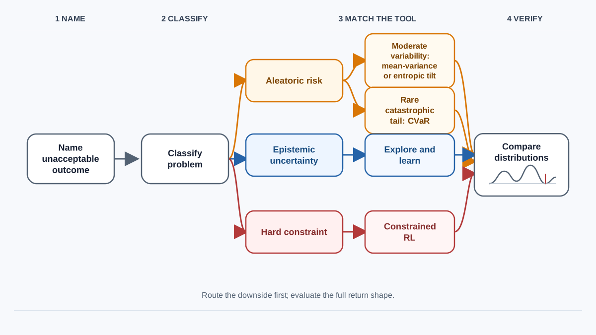
Here is the sequence I use when deciding whether and how to go risk-sensitive:

Step one: name the unacceptable outcome. Be specific. Is it a 10% drop in average performance? A 1-in-100 catastrophic episode? A hard behavioral limit? Write down what you cannot tolerate and how often you cannot tolerate it.

Step two: classify it. Is the problem aleatoric risk, epistemic uncertainty, or a hard constraint? Route accordingly. Risk-sensitive objective for aleatoric variability. Exploration for ignorance. Constrained RL for forbidden behavior.

Step three: match the objective to the failure shape. Consistent but moderate degradation: mean-variance or a mild entropic tilt. Rare catastrophic tail: CVaR. Hard limit: constraint, not risk measure.

Step four: verify empirically. Do not trust the objective choice on faith. Run the same environment under a mean objective and your chosen risk-sensitive objective, then compare the full return distributions of the resulting policies—not just their means.

Before you run the comparison, declare your evaluation criteria. Choose the tail level or failure threshold up front, and commit to the statistics you will compare: mean, the selected quantile or CVaR, the probability of crossing your unacceptable threshold, and variability across episodes. Then run enough evaluation episodes to support the conclusion.

Warning: Rare-event tails are exactly where finite samples are weakest. A lower observed tail can reflect sampling noise rather than a real policy improvement. If your unacceptable outcome occurs in 1% of episodes, you need enough evaluation coverage to estimate that 1% reliably—and you need repeated seeds to confirm the effect is not an artifact of one lucky or unlucky run.

This last step is where the conceptual choice becomes an observable fact. A risk-sensitive objective is a hypothesis about which part of the return distribution matters. The experiment is how you test it. Run both policies, collect the full distribution of returns from each, and look at the tails with your own eyes. The mean-optimal policy and the risk-sensitive policy will often have similar averages. The difference will be visible in the shape of the distribution—and that shape is the entire point.

If the risk-sensitive policy does not visibly avoid the outcome you feared, you have learned something useful: either the objective does not match your downside shape, the tail level was set incorrectly, or the estimation quality is insufficient to resolve the tail. Adjust the objective, tighten the evaluation, and run the comparison again. That iteration is not a failure of the method. It is the method working as intended.

References

Research updated Sep 9, 2026