
Compare Penalty and Primal-Dual Methods in a Small Constrained MDP
A hand-picked penalty weight can look fine in one run and drift over budget in the next. The weight was never told what the budget is — so it can't respect…

Key topics
A hand-picked penalty weight can look fine in one run and drift over budget in the next. The weight was never told what the budget is — so it can't respect it.
Here is the smallest experiment I know that exposes the difference between discouraging cost and constraining it: one toy gridworld, two methods, one budget line on a chart.
We'll build a tabular constrained MDP in Python, run a fixed-penalty baseline, then run a Lagrangian primal-dual method that updates a nonnegative multiplier from the observed cost-budget gap. Then we'll read the results honestly — because "my mean cost was under budget" and "my policy is safe" are not the same sentence.
If you already know the environment contract and repeated-episode evaluation, you're set. If not, the short version: an environment hands back a state and two signals per step, and you judge a policy by averaging over many episodes from a start-state distribution, not by one lucky trajectory.
The Toy Problem: A Gridworld With a Cost Channel
We'll use a 5×5 grid. The agent starts top-left, the goal is bottom-right, and a hazard region sits in the middle. Episodes end at the goal or after a short horizon.
Two signals per step, kept in separate arrays:
- Reward:
-0.01per step (a small living cost),+1.0on reaching the goal. - Cost:
1.0when the agent steps into a hazard cell,0.0otherwise.
import numpy as np

GRID = 5
HAZARD = {(1, 1), (1, 2), (2, 2), (3, 1)}
GOAL = (4, 4)
HORIZON = 40
ACTIONS = [(-1, 0), (1, 0), (0, -1), (0, 1)]  # up, down, left, right

def step(state, action):
    r, c = state
    dr, dc = ACTIONS[action]
    nr, nc = min(max(r + dr, 0), GRID - 1), min(max(c + dc, 0), GRID - 1)
    nxt = (nr, nc)
    reward = 1.0 if nxt == GOAL else -0.01
    cost = 1.0 if nxt in HAZARD else 0.0
    done = nxt == GOAL
    return nxt, reward, cost, done
The constraint is a budget on mean episodic cost: across the evaluation distribution, average cost per episode must stay at or below B. We'll set B = 2.0.
Why episodes and not steps? Because a single trajectory is one sample. A per-step rule ("never enter a hazard") is a different, stronger specification — and it's not what we're testing. We're testing whether the expected cost of the policy stays under a line. That's a statement about a distribution, and you can only check it by sampling from that distribution repeatedly.
Note: Keep cost out of the reward array at the environment level. The moment you fold cost into reward inside
step(), you've made an algorithmic choice inside your simulator, and you can no longer compare methods cleanly.
Knowledge check
Check your understanding
Answer this question before you continue.
Two Ways to Respect a Budget
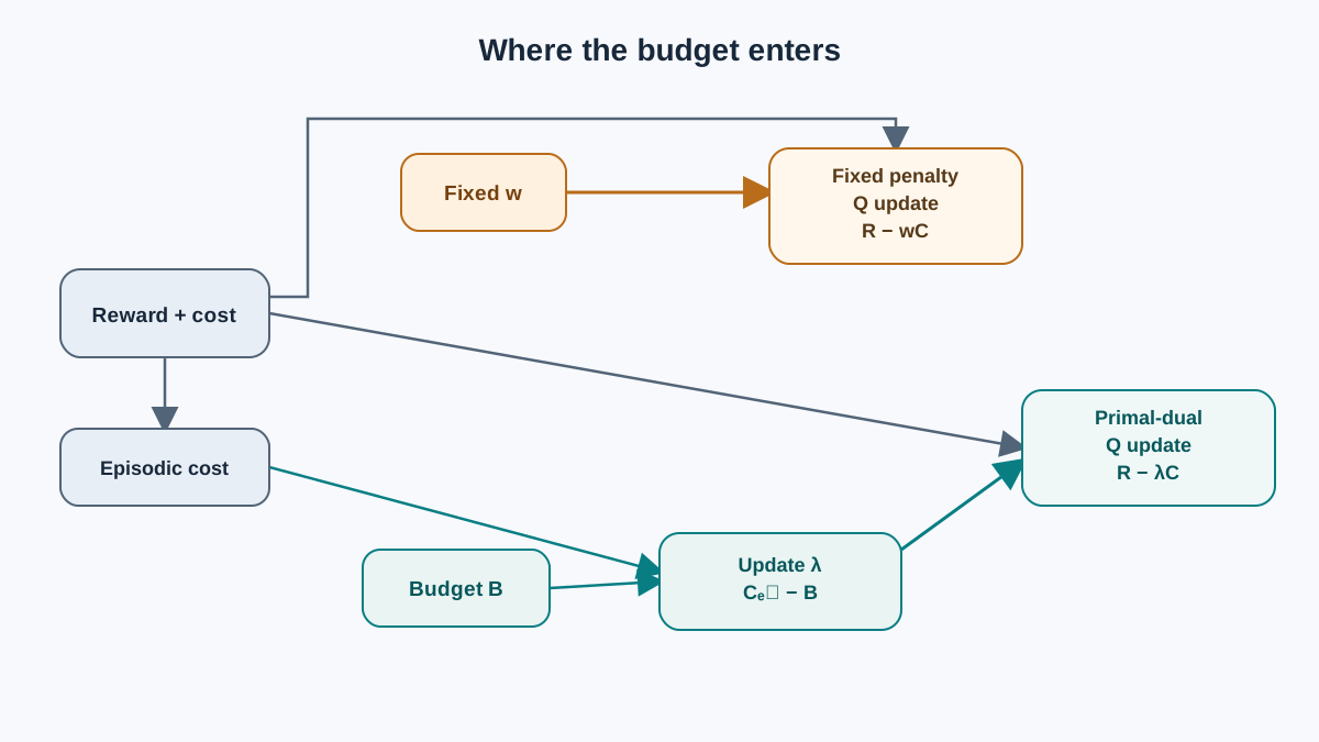
Before the code, the mechanism. Both methods use the same Q-learning core. They differ in what the agent optimizes.
| Fixed penalty | Primal-dual (Lagrangian) | |
|---|---|---|
| Objective | r - w * c | r - λ * c |
| Key parameter | w, chosen by hand | λ, updated from data |
| Budget used? | No — only w | Yes — λ moves on the cost-budget gap |
| What it promises | Soft preference for low cost | Soft preference, adaptively tuned |
| Guarantee during training | None | None |
The structural difference is the exchange rate. A penalty has a fixed exchange rate between reward and cost: one unit of cost always costs you w units of reward. A multiplier has an adaptive one: it rises when the agent is over budget and falls when it's under.
Neither method, as implemented here, guarantees safety during training. Feasibility is something we measure afterward, not something the loop enforces. That boundary matters, and I'd rather state it up front than let the chart imply more than it proves.
Baseline: Fixed Penalty Q-Learning
Standard tabular Q-learning, with the shaped reward r - w * c and w picked by hand. The mode is explicit: pass w for a fixed penalty, or pass lam and budget for the primal-dual run.
def q_learning(env_step, episodes, alpha=0.1, gamma=0.95,
               epsilon=0.1, w=None, lam=None, budget=None, eta=0.0):
    Q = np.zeros((GRID, GRID, len(ACTIONS)))
    log = {"reward": [], "cost": [], "lam": []}
    primal_dual = lam is not None and budget is not None
    if primal_dual:
        lam = float(lam)
    else:
        w = 0.0 if w is None else float(w)

    for ep in range(episodes):
        state, done, ep_r, ep_c = (0, 0), False, 0.0, 0.0
        for _ in range(HORIZON):
            if np.random.rand() < epsilon:
                a = np.random.randint(len(ACTIONS))
            else:
                a = int(np.argmax(Q[state[0], state[1]]))

            nxt, r, c, done = env_step(state, a)
            weight = lam if primal_dual else w
            shaped = r - weight * c
            target = shaped + gamma * np.max(Q[nxt[0], nxt[1]]) * (not done)
            Q[state[0], state[1], a] += alpha * (target - Q[state[0], state[1], a])

            state = nxt
            ep_r += r
            ep_c += c
            if done:
                break

        log["reward"].append(ep_r)
        log["cost"].append(ep_c)
        log["lam"].append(lam if primal_dual else 0.0)

        if primal_dual:
            lam = max(0.0, lam + eta * (ep_c - budget))

    return Q, log
Two things to notice. First, we log undiscounted episodic reward and undiscounted episodic cost separately. If you only log the shaped return, the cost signal disappears into the penalty and you can't check the budget. Second, the penalty branch never reads budget. That's the point.
Run it with w=0.0, w=0.5, and w=2.0 and look at mean cost over the last 100 episodes:
for w in [0.0, 0.5, 2.0]:
    _, log = q_learning(step, episodes=2000, w=w)
    print(f"w={w}: mean cost={np.mean(log['cost'][-100:]):.2f}, "
          f"mean reward={np.mean(log['reward'][-100:]):.2f}")
You'll see mean cost land on different sides of B = 2.0 depending on w. That's the failure mode in one line of output: the agent respects the weight, not the budget. A penalty can be tuned to sit near the budget, but the tuning is manual and the result is a soft preference.
Knowledge check
Check your understanding
Answer this question before you continue.
Primal-Dual: Let the Multiplier Find the Budget
Same environment, same Q-learning core. Two changes: the objective uses λ instead of w, and λ gets its own update.
The Lagrangian objective per step is r - λ * c. The dual update is:
lam = max(0.0, lam + eta * (ep_c - budget))
Over budget pushes λ up. Under budget pushes it down. The clamp keeps λ nonnegative, because a negative multiplier would reward cost — the opposite of what we want. That's the whole mechanism.
_, log = q_learning(step, episodes=2000, lam=0.0, budget=2.0, eta=0.05)
print(f"final lambda={log['lam'][-1]:.2f}")
print(f"mean cost={np.mean(log['cost'][-100:]):.2f}")
print(f"mean reward={np.mean(log['reward'][-100:]):.2f}")
Expected shape of the output: λ starts at zero, rises while the agent is over budget, and settles somewhere that keeps mean cost near the line. You should be able to watch λ doing the work the hand-tuned w did in the baseline — except nobody told it the answer.
Three mistakes I see in almost every first implementation:
Common mistake: Forgetting the
max(0.0, ...)clamp. Without it,λgoes negative when the agent is comfortably under budget, and the objective starts paying the agent to collect cost.Common mistake: Updating
λevery step instead of every episode. The dual variable is supposed to respond to episodic cost against an episodic budget. Per-step updates make the multiplier chase noise.Common mistake: Mixing a discounted cost into the dual update while reporting undiscounted episodic cost. Pick one convention and use it in both places, or your budget line and your update rule are measuring different things.
There's also a second learning rate now: eta for the multiplier, alongside alpha for Q-values. eta is a real tuning knob. Set it too high and λ oscillates around the budget instead of settling.
Knowledge check
Check your understanding
Answer this question before you continue.
Reading the Results Without Fooling Yourself
One run is an anecdote. Run both methods across several seeds and report mean episodic cost with spread.
The critical detail: evaluate the learned policy separately, with exploration disabled. The training log includes exploratory actions, so its final episodes are not a clean measurement of what the policy learned. After training, run the greedy policy on a fixed set of evaluation episodes and measure cost there.
def evaluate(Q, episodes=100):
    rewards, costs = [], []
    for _ in range(episodes):
        state, done, ep_r, ep_c = (0, 0), False, 0.0, 0.0
        for _ in range(HORIZON):
            a = int(np.argmax(Q[state[0], state[1]]))  # no exploration
            state, r, c, done = step(state, a)
            ep_r += r
            ep_c += c
            if done:
                break
        rewards.append(ep_r)
        costs.append(ep_c)
    return np.array(rewards), np.array(costs)

def run_seeds(method, seeds=10, episodes=2000):
    costs, rewards = [], []
    for s in range(seeds):
        np.random.seed(s)
        if method == "penalty":
            Q, _ = q_learning(step, episodes=episodes, w=0.5)
        else:
            Q, _ = q_learning(step, episodes=episodes,
                              lam=0.0, budget=2.0, eta=0.05)
        r, c = evaluate(Q)
        costs.append(c.mean())
        rewards.append(r.mean())
    return np.array(costs), np.array(rewards)

for m in ["penalty", "primal-dual"]:
    c, r = run_seeds(m)
    print(f"{m}: cost {c.mean():.2f} ± {c.std():.2f}, "
          f"reward {r.mean():.2f} ± {r.std():.2f}")
The comparison that matters is mean episodic cost against the budget line, side by side, over the same evaluation episodes. If the primal-dual mean sits at or below 2.0 across the seeds you ran, you have empirical feasibility: a statement about your sample, not a proof about the policy.
What would a formal guarantee require? Convergence conditions on the step sizes, assumptions about the MDP that this toy doesn't satisfy, and a proof that the primal-dual iterates reach a saddle point. The safe-RL literature is careful about this for a reason — primal-dual methods can be unstable, and safety during training is not guaranteed by the update rule alone. Don't claim a guarantee from this code.
Warning: The primal-dual method here is tabular and small-scale. The multiplier behavior you observe is real, but the convergence story does not transfer automatically to function approximation. A neural policy changes the problem; it doesn't just scale the same one.
Knowledge check
Check your understanding
Answer this question before you continue.
One Modification Worth Trying
Change the budget. Set B = 1.0, then B = 3.0, and rerun both methods.
The penalty baseline needs you to re-tune w by hand to track the new budget — and you'll have to guess again. The primal-dual method should move λ on its own, because λ is driven by the measured gap between episodic cost and the budget you actually stated.
That asymmetry is the whole article. The multiplier encodes the budget; the penalty weight encodes a guess.
A second variation: tighten eta from 0.05 to 0.01 and watch the oscillation around the budget shrink. Then push it to 0.2 and watch it grow. Record mean episodic cost, mean episodic reward, and final λ for each setting so the comparison stays honest across changes.
Where This Leaves You
Use a fixed penalty when you can afford to hand-tune the tradeoff and you only need to discourage cost. Reach for a multiplier when the budget itself is the specification and you want the algorithm to respond to measured violation.
Both are empirical here. Neither guarantees safety during training. The multiplier is the budget made visible in code — a live number that rises when you're over the line and falls when you're under.
Your next step: take this same loop and swap the gridworld for a slightly larger or continuous environment, keeping the reward and cost channels separate. Watch what happens to λ when the state space stops fitting in a table. That's where the honest questions about function approximation and stability begin.
Knowledge check
Final check
Finish the article by checking the ideas you just learned.
References
Build a stronger RL mental model
Use structured resources to connect equations, algorithms, and observable agent behavior.


