
Compare Offline Policy-Value Estimates on Logged Trajectories
Two estimators, one dataset, two different answers. That gap is not a bug in the math — it is the most useful signal you will get about whether your logs…

Key topics
Two estimators, one dataset, two different answers. That gap is not a bug in the math — it is the most useful signal you will get about whether your logs can answer the question you are asking.
This is a hand-computation drill backed by a short runnable script. The dataset is small enough to check with a calculator, which means you can see exactly where variance and model dependence enter. I have watched people run off-policy evaluation libraries for months without ever building this intuition, and it costs them: they report a number, someone asks how stable it is, and they have nothing to say.
We will compute three estimates — importance sampling, direct method, and doubly robust — on the same logged trajectories, then compare them.
The Dataset You Will Work With
A tiny environment: three states, two actions (A and B), episodes of exactly three steps, discount factor γ = 1.0 so the arithmetic stays clean. The behavior policy that generated the logs is deliberately uneven — it favors action A almost everywhere.
Behavior policy π_b:
| State | P(A) | P(B) |
|---|---|---|
| s1 | 0.9 | 0.1 |
| s2 | 0.8 | 0.2 |
| s3 | 0.5 | 0.5 |
Target policy π_e (the one we want to evaluate):
| State | P(A) | P(B) |
|---|---|---|
| s1 | 0.2 | 0.8 |
| s2 | 0.3 | 0.7 |
| s3 | 0.5 | 0.5 |
The target policy prefers B; the behavior policy mostly chose A. That mismatch is the whole point of the exercise.
Logged trajectories (five episodes, each with the behavior probability of the taken action):
| # | Step | State | Action | Reward | π_b(a|s) |
|---|---|---|---|---|---|
| 1 | 1 | s1 | A | 1 | 0.9 |
| 1 | 2 | s2 | A | 2 | 0.8 |
| 1 | 3 | s3 | A | 1 | 0.5 |
| 2 | 1 | s1 | A | 1 | 0.9 |
| 2 | 2 | s2 | B | 3 | 0.2 |
| 2 | 3 | s3 | A | 1 | 0.5 |
| 3 | 1 | s1 | B | 2 | 0.1 |
| 3 | 2 | s2 | A | 2 | 0.8 |
| 3 | 3 | s3 | B | 4 | 0.5 |
| 4 | 1 | s1 | A | 1 | 0.9 |
| 4 | 2 | s2 | A | 2 | 0.8 |
| 4 | 3 | s3 | A | 1 | 0.5 |
| 5 | 1 | s1 | A | 1 | 0.9 |
| 5 | 2 | s2 | A | 2 | 0.8 |
| 5 | 3 | s3 | A | 1 | 0.5 |
Assumptions, stated plainly: finite horizon, behavior probabilities known exactly (not estimated), and overlap — every action the target policy can take has nonzero probability under the behavior policy. Trajectory 3 is the interesting one. It is the only episode where the behavior policy took action B at s1, and it is the only episode with a large reward at s3.
If the reweighting logic feels shaky, the intuition is worth one sentence: importance sampling re-weights each logged trajectory by how much more (or less) likely the target policy was to produce it, so the weighted average estimates the target policy's value.
Compute the Importance-Sampling Estimate
For each trajectory, the weight is the product of per-step ratios π_e(a|s) / π_b(a|s) across the episode.
Trajectory 1 (A, A, A):
- s1: 0.2 / 0.9 = 0.2222
- s2: 0.3 / 0.8 = 0.3750
- s3: 0.5 / 0.5 = 1.0000
- Weight = 0.2222 × 0.3750 × 1.0 = 0.0833
- Return = 1 + 2 + 1 = 4
- Weighted return = 0.0833 × 4 = 0.333
Trajectory 2 (A, B, A):
- s1: 0.2222, s2: 0.7 / 0.2 = 3.5, s3: 1.0
- Weight = 0.2222 × 3.5 × 1.0 = 0.7778
- Return = 1 + 3 + 1 = 5
- Weighted return = 0.7778 × 5 = 3.889
Trajectory 3 (B, A, B):
- s1: 0.8 / 0.1 = 8.0, s2: 0.375, s3: 1.0
- Weight = 8.0 × 0.375 × 1.0 = 3.0
- Return = 2 + 2 + 4 = 8
- Weighted return = 3.0 × 8 = 24.0
Trajectory 4 (A, A, A): same as trajectory 1 — weight 0.0833, weighted return 0.333
Trajectory 5 (A, A, A): same again — weighted return 0.333
Standard IS estimate = average of weighted returns:
(0.333 + 3.889 + 24.0 + 0.333 + 0.333) / 5 = 28.888 / 5 = 5.78
Self-normalized IS divides by the sum of weights instead of the count:
Sum of weights = 0.0833 + 0.7778 + 3.0 + 0.0833 + 0.0833 = 4.028 SNIS = 28.888 / 4.028 = 7.17
Two estimators, same data, answers of 5.78 and 7.17. Hold both numbers. The gap is the first warning sign.
Knowledge check
Check your understanding
Answer this question before you continue.
Where the Variance Comes From
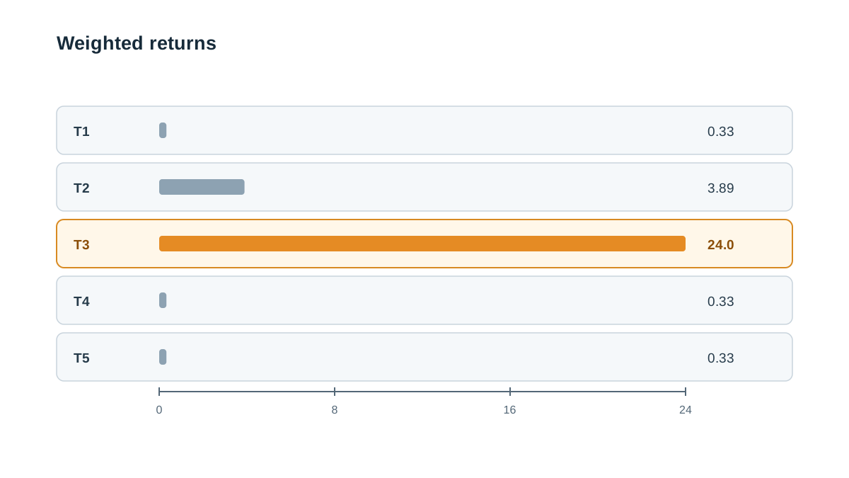
Look at the weighted returns again: 0.333, 3.889, 24.0, 0.333, 0.333.
One trajectory contributes 24.0. The other four contribute 4.9 combined. Trajectory 3 is not a data point in this average — it is the average. Remove it and the IS estimate collapses to 0.97.
The mechanism is compounding. Each per-step ratio multiplies into the next, so a single low-probability action under the behavior policy inflates the whole trajectory's weight. Trajectory 3 hit a 0.1-probability action at s1 and paid for it with a weight of 8.0 before the other steps even contributed. Longer episodes make this worse: ratios compound multiplicatively, so weight variance grows roughly exponentially in horizon length.
A crude spread measure makes the instability visible. The range of weighted returns is 24.0 − 0.333 = 23.7, and the standard deviation is roughly 9.4 — larger than the estimate itself.
Weight clipping is the standard mitigation. Cap every weight at some threshold c and recompute. With c = 1.0:
- Trajectory 3's weight drops from 3.0 to 1.0, weighted return 8.0
- New sum of weighted returns = 0.333 + 3.889 + 8.0 + 0.333 + 0.333 = 12.888
- Clipped IS = 12.888 / 5 = 2.58
The estimate fell from 5.78 to 2.58. Clipping buys stability by accepting bias — you are deliberately under-weighting the trajectories the target policy loves most. That trade is often worth it, but you should know you made it.
Common mistake: Treating "unbiased" as "trustworthy." Standard IS is unbiased in expectation over infinitely many datasets. You have five trajectories. Unbiasedness is a statement about a distribution you will never observe; your estimate is one draw from it.
Knowledge check
Check your understanding
Answer this question before you continue.
Build a Direct-Method Value Model
The direct method skips reweighting entirely. Instead, you model the expected return of each state-action pair — a Q-estimate — and average those predictions under the target policy.
Here is the trap that breaks most hand-worked DR examples, including the first version of this one. If you estimate Q(s, a) from the full-episode return of trajectories that happened to pass through (s, a), you are mixing two different quantities: the return from the start of the episode and the return from state s onward. Those are not the same number, and averaging them across states as if each state were equally likely is not the target policy's value either.
The clean fix is to define one estimand and stick to it. Let the value we want be the expected return from the start state s1 under the target policy. Then the direct method needs exactly one prediction: the expected return of the target policy's first action at s1, plus the continuation. For a three-step episode with γ = 1, that is the full-episode return.
So the model only has to answer one question: what return does the target policy get starting from s1?
From the logs, the two candidate first actions are A and B. Estimate each from the trajectories that actually took it:
| First action at s1 | Trajectories | Mean return | Q-estimate |
|---|---|---|---|
| A | 1, 2, 4, 5 | (4 + 5 + 4 + 4) / 4 | 4.25 |
| B | 3 | 8 / 1 | 8.00 |
The direct-method estimate is the target policy's weighted average over these two first actions:
DM = 0.2 × 4.25 + 0.8 × 8.00 = 0.85 + 6.40 = 7.25
Now perturb one value. Change Q(s1, B) from 8.00 to 4.25 — a plausible correction if you suspect trajectory 3's reward was lucky:
DM = 0.2 × 4.25 + 0.8 × 4.25 = 4.25
A single Q-value moved the estimate by three full points. That is model sensitivity in one line of arithmetic. And notice the deeper problem: Q(s1, B) is estimated from exactly one trajectory. The model is not just sensitive — it is confidently wrong about how much it knows.
Warning: A direct-method model that looks clean on paper can be extrapolating from a single logged transition. When the logs barely cover a state-action pair, the model's confidence is an artifact of the fitting procedure, not evidence.
Knowledge check
Check your understanding
Answer this question before you continue.
Combine Them Into a Doubly Robust Estimate
The doubly robust estimator uses the model as a baseline and lets importance weights correct the residual between what actually happened and what the model predicted.
Because our estimand is the return from s1, the residual is defined at the same level: observed full-episode return minus the model's prediction for the first action taken. The weight is the full-trajectory ratio, exactly as in the IS section.
The form: DM estimate + importance-weighted average of (observed return − model prediction).
| # | First action | Return | Model prediction | Residual | Weight | Weighted residual |
|---|---|---|---|---|---|---|
| 1 | A | 4 | 4.25 | −0.25 | 0.0833 | −0.021 |
| 2 | A | 5 | 4.25 | 0.75 | 0.7778 | 0.583 |
| 3 | B | 8 | 8.00 | 0.00 | 3.0 | 0.000 |
| 4 | A | 4 | 4.25 | −0.25 | 0.0833 | −0.021 |
| 5 | A | 4 | 4.25 | −0.25 | 0.0833 | −0.021 |
Weighted residual term = (−0.021 + 0.583 + 0.000 − 0.021 − 0.021) / 5 = 0.104
DR estimate = 7.25 + 0.104 = 7.35
The mechanism is visible in the table. Trajectory 3 got a weight of 3.0, but its residual was zero — the model already predicted that return, so the heavy weight had nothing to amplify. Trajectory 2 carried the correction instead, with a modest weight of 0.78.
That is the DR promise: when the model is good, residuals are small and the variance stays low even with uneven weights. When the model is bad, the weights carry the correction.
But the promise has a hole. If the model is misspecified and the weights are heavy, DR can be worse than both components. The model's error gets amplified by the same weights that were supposed to fix it. This is not a theoretical edge case; it is the normal failure mode on datasets with poor coverage.
Knowledge check
Check your understanding
Answer this question before you continue.
Run It Yourself
Hand arithmetic catches conceptual errors. Code catches bookkeeping errors — and once you have more than a handful of trajectories, bookkeeping is where the bugs live. Here is the whole exercise in the standard library, no dependencies:
import math

# (state, action, reward, behavior_prob) per step, one list per trajectory
trajectories = [
    [("s1","A",1,0.9), ("s2","A",2,0.8), ("s3","A",1,0.5)],
    [("s1","A",1,0.9), ("s2","B",3,0.2), ("s3","A",1,0.5)],
    [("s1","B",2,0.1), ("s2","A",2,0.8), ("s3","B",4,0.5)],
    [("s1","A",1,0.9), ("s2","A",2,0.8), ("s3","A",1,0.5)],
    [("s1","A",1,0.9), ("s2","A",2,0.8), ("s3","A",1,0.5)],
]

target = {"s1": {"A":0.2,"B":0.8}, "s2": {"A":0.3,"B":0.7}, "s3": {"A":0.5,"B":0.5}}

def weight(traj):
    w = 1.0
    for s, a, _, pb in traj:
        w *= target[s][a] / pb
    return w

def ret(traj):
    return sum(r for _, _, r, _ in traj)

weights = [weight(t) for t in trajectories]
returns = [ret(t) for t in trajectories]
weighted = [w * g for w, g in zip(weights, returns)]

is_est = sum(weighted) / len(weighted)
snis_est = sum(weighted) / sum(weights)

# Direct method: Q(s1, A) and Q(s1, B) from mean return of trajectories taking that action
q = {}
for action in ("A", "B"):
    rs = [ret(t) for t in trajectories if t[0][1] == action]
    q[action] = sum(rs) / len(rs)
dm_est = target["s1"]["A"] * q["A"] + target["s1"]["B"] * q["B"]

# Doubly robust: DM baseline + weighted mean residual at the first action
residuals = [g - q[t[0][1]] for t, g in zip(trajectories, returns)]
dr_est = dm_est + sum(w * r for w, r in zip(weights, residuals)) / len(trajectories)

print(f"weights:        {[round(w, 4) for w in weights]}")
print(f"IS:             {is_est:.2f}")
print(f"SNIS:           {snis_est:.2f}")
print(f"DM:             {dm_est:.2f}")
print(f"DR:             {dr_est:.2f}")
print(f"weight mass:    {sum(weights):.3f}")
print(f"top weight share: {max(weights) / sum(weights):.1%}")
Expected output:
weights:        [0.0833, 0.7778, 3.0, 0.0833, 0.0833]
IS:             5.78
SNIS:           7.17
DM:             7.25
DR:             7.35
weight mass:    4.028
top weight share: 74.5%
Two checks worth running before you trust any of it. First, the weighted returns should sum to is_est * len(weighted) — if they do not, your weight function is wrong. Second, the top weight share should match your hand calculation. Here it is 74.5%, which means trajectory 3 alone carries nearly three quarters of the total weight mass. That single number is the whole variance story.
Common mistake: Computing the DR residual against a model prediction for a different state than the one the weight was computed for. The residual and the weight must describe the same decision point, or the correction is meaningless.
Compare the Three Estimates Side by Side
| Estimator | Value | Rough variance | Depends on |
|---|---|---|---|
| IS | 5.78 | Very high (SD ≈ 9.4) | Behavior probabilities only |
| SNIS | 7.17 | High | Behavior probabilities only |
| Direct method | 7.25 | Low | Model correctness |
| Doubly robust | 7.35 | Moderate | Both, with correction |
The estimates disagree. IS says 5.78; SNIS says 7.17; DM says 7.25; DR says 7.35. That disagreement is a diagnostic, not noise to average away. When estimators that rely on different assumptions land in different places, at least one assumption is being violated.
My decision rule: trust the estimate only when the estimators roughly agree and no single trajectory dominates the weight distribution. Here, the spread from 5.78 to 7.35 is too wide, and trajectory 3's weight of 3.0 against a sum of 4.03 means one episode controls nearly three quarters of the total weight mass. I would not report any of these numbers as the value of the target policy.
To see the divergence grow, tighten the target policy toward B at s1 — say P(B) = 0.95. The ratio at s1 jumps from 8.0 to 9.5, trajectory 3's weight climbs to 3.56, and the IS estimate swings further while the direct method barely moves. As overlap shrinks, the estimators stop agreeing.
When the Logs Cannot Answer the Question
Support means the target policy places probability only where the behavior policy also placed probability. Formally: if π_b(a|s) = 0, then π_e(a|s) must also be 0. Otherwise the ratio is undefined and the estimate is meaningless.
Here is the failure case. Suppose the target policy assigns P(B|s2) = 0.7, but the logs contain no trajectory where B was taken at s2 under a behavior policy that could not have chosen it. If π_b(B|s2) = 0, the weight is 0.7 / 0 — undefined. No estimator fixes this. IS cannot reweight a trajectory that does not exist. The direct method will happily extrapolate from neighboring states and return a confident number. DR will inherit that confident number and dress it in a correction term that has nothing to correct.
No estimator can fix a coverage gap. It can only hide it behind a confident-looking number.
Practical checks before you trust any estimate — treat these as illustrative flags, not universal thresholds:
- Count trajectories per state-action pair. In this dataset, (s1, B) has exactly one observation. That is a support risk, and it is why the DM estimate is fragile.
- Report the maximum normalized weight. Here it is 74.5%. When one trajectory carries most of the weight mass, the estimate is hostage to that trajectory.
- Flag states where the target and behavior policies diverge sharply. The ratio at s1 is 8.0. That is the source of the weight concentration, and it is worth naming explicitly.
- Re-run with a clipped weight and compare. Clipping at c = 1.0 moved the IS estimate from 5.78 to 2.58 — a 55% shift. A shift that large means the unclipped number was never stable, and the right response is more data or an uncertainty interval, not a tighter cutoff.
The dataset-support question — whether your logs can identify the target policy's value at all — is a separate diagnostic from estimator choice. Coverage is a property of the data; variance is a property of the estimator. You need both to be sound.
Your Turn: Change One Thing
Shrink the behavior policy's probability on action B at s1 from 0.1 to 0.05. Recompute all three estimates before reading further.
Predict first. Which estimator moves most?
The IS estimate should swing hardest. Trajectory 3's weight at s1 doubles from 8.0 to 16.0, pushing its trajectory weight from 3.0 to 6.0 and its weighted return from 24.0 to 48.0. The new IS estimate roughly doubles. The direct method does not move at all — it never looks at behavior probabilities. DR lands between them: the residual term grows because trajectory 3's weight grew, but the model baseline anchors the estimate.
That pattern — IS swings, DM holds, DR splits the difference — is the signature of weight inflation. When you see it, you are watching variance, not signal.
Second variation: clip the weights at c = 1.0 and recompute. The estimate shifts toward the direct method, because clipping suppresses exactly the trajectories the target policy favors most. That shift is the bias you accepted in exchange for stability.
The next step is scaling this computation to a real logged dataset: compute the weight distribution, plot it, and check whether the top few trajectories dominate. If they do, you have a support problem, not an estimator problem — and no amount of estimator sophistication will fix it.
Knowledge check
Final check
Finish the article by checking the ideas you just learned.
References
Build a stronger RL mental model
Use structured resources to connect equations, algorithms, and observable agent behavior.


