Importance Sampling and Doubly Robust Evaluation in Offline RL

You have a dataset of logged trajectories collected under one policy, and you want to know what a different policy would have earned. The naive fix—reweighting each trajectory by how much more likely the target policy would have taken those actions—is unbiased in theory and explosive in practice. The real design question is not which formula to apply, but how much model you trust to buy back variance.

Why Logged Data Cannot Answer Directly

Every trajectory in your dataset carries the fingerprints of the policy that collected it. The states visited, the actions attempted, the rewards received—all of it was shaped by the behavior policy's preferences. When you average the returns in that dataset, you are estimating the behavior policy's value, not the target policy's.

This is the off-policy evaluation problem in its simplest form. You want the answer to a counterfactual question: what would have happened if a different policy had been in control? The logs cannot answer that question directly because they never show you the counterfactual. They only show you what one particular policy actually did.

The gap between the behavior policy and the target policy is the entire reason estimators exist. If the two policies were identical, you would just average the logged returns and be done. The moment they diverge, every naive average inherits the behavior policy's biases.

If you have worked through the off-policy evaluation workflow and understand dataset coverage, you already know the shape of the problem. What follows is the correction mechanism itself.

The Importance Weight: Correcting for Whose Hand Chose the Action

Imagine a single decision point. The behavior policy chose action a in state s with probability 0.2. The target policy you want to evaluate would have chosen that same action with probability 0.8. That logged action is more representative of what the target policy would do than the behavior policy's odds suggest—so it deserves more weight.

The importance weight is a likelihood ratio: how much more (or less) likely the target policy was to pick the action that actually happened.

weight = P_target(action | state) / P_behavior(action | state)

Actions the target policy would rarely take get downweighted. Actions it would favor get upweighted. A trajectory where the target policy would have made the same choices as the behavior policy receives a weight near 1. A trajectory full of actions the target policy would never choose receives a weight near 0.

But a trajectory is not a single decision. It is a chain of them. The probability that the target policy would have produced the entire trajectory is the product of its per-step action probabilities. The same is true for the behavior policy. So the trajectory-level importance weight is the product of per-step ratios:

trajectory_weight = Π_t P_target(a_t | s_t) / P_behavior(a_t | s_t)

The product appears because every decision had to happen for the trajectory to unfold as it did. If the target policy would have balked at any single action, the whole path becomes less representative.

Consider a two-step trajectory. The behavior policy chose action a₁ in state s₁, then action a₂ in state s₂. The target policy would have chosen a₁ with probability 0.9 (vs. 0.5 for the behavior policy) and a₂ with probability 0.7 (vs. 0.4). The trajectory weight is (0.9/0.5) × (0.7/0.4) = 1.8 × 1.75 = 3.15. This trajectory was more than three times as likely under the target policy, so it gets amplified accordingly.

This is the core mechanism of importance sampling off-policy evaluation: reweight logged experience so that it reads like samples from the target policy's distribution.

Use the trajectory-level product of the per-step ratios.

Why Ordinary Importance Sampling Is Unbiased but Noisy

Here is where the first instinct quietly breaks.

The ordinary importance sampling estimator averages the weighted returns across all logged trajectories. In expectation, that average converges to the target policy's true value. Unbiased means correct on average across many datasets—not correct on any single estimate.

The variance tells a different story. It scales with how far the target policy strays from the behavior policy. When the two policies are close, the weights hover near 1 and the estimator behaves. When they diverge, the weights spread out, and the estimator starts to rattle.

Long horizons compound the problem. The product of per-step weights multiplies small divergences into large swings. A target policy that differs modestly from the behavior policy at every step can produce trajectory weights that vary by orders of magnitude over a 50-step horizon. Research on marginalized importance sampling has shown that this variance can grow exponentially with the horizon—the cumulative product of weights becomes a volatility amplifier.

A single trajectory with a huge weight can dominate the entire estimate. One rare event under the behavior policy that the target policy would have pursued eagerly can carry more influence than hundreds of ordinary trajectories combined. The point estimate can look absurd—a value far outside any plausible range—even though the method is theoretically correct.

This is the uncomfortable truth about ordinary importance sampling: it is unbiased in expectation and unusable in practice whenever the policies diverge meaningfully or the horizon runs long.

Weighted Importance Sampling: Trading Bias for Stability

The first practical correction is almost embarrassingly simple: divide by the sum of the weights instead of the number of trajectories.

Ordinary importance sampling treats every trajectory as one observation, scaled by its weight. Weighted importance sampling normalizes the weights so they sum to 1. A trajectory with a weight of 100 no longer contributes 100 times a normal trajectory's influence—it contributes 100/Σw, which is bounded by 1.

This caps the leverage of any single outlier trajectory. The variance drops, often dramatically.

The cost is bias. The weighted estimator is no longer unbiased in expectation. It converges to the correct value as the dataset grows, but for finite data it leans slightly toward the behavior policy's region of experience. The bias shrinks as you add trajectories, but it never quite disappears.

When the behavior and target policies are close, the two estimators nearly agree. The weights cluster near 1, so normalizing by their sum barely changes anything. When the policies diverge, the difference becomes visible: ordinary importance sampling swings wildly around the true value, while weighted importance sampling stays calmer but sits slightly off.

For finite logged datasets, weighted importance sampling is usually the safer default. A small, bounded bias beats a variance that can make your estimate meaningless.

Doubly Robust Estimation: Borrowing a Model to Cut Variance

Weighted importance sampling reduces variance by capping outlier influence, but it still relies entirely on the logged trajectories. There is another source of information you have not used yet: a learned model of the environment.

The direct method takes that path. Learn a value model from the logged data—a function that predicts expected return from any state under any policy—and evaluate the target policy by querying the model. This approach has low variance: the model produces smooth predictions regardless of policy divergence. But it is biased whenever the model is wrong, and models learned from logged data are wrong in exactly the regions where the target policy strays from the behavior policy's coverage.

Doubly robust estimation combines both approaches. It starts from the model's prediction and adds an importance-weighted correction only for the part the model missed.

estimate = model_prediction + importance_weight × (observed_return − model_prediction)

Think of the model as a prior guess and the importance weight as a correction applied only to the residual—the difference between what the model predicted and what actually happened. If the model is accurate, the residual is small, the correction term is small, and the variance stays low. If the model is wrong, the importance weights still correct the bias, because the residual carries the full error.

This is the "doubly" in doubly robust: the estimator leans on two sources of information and only needs one to be reliable. If the model is accurate, you get low variance. If the model is wrong but the importance weights are correct, you still get an unbiased estimate. The estimator is consistent if either the model or the weights are right.

The Real Tradeoff: Model Dependence vs. Variance

Doubly robust estimation is not free. It inherits the direct method's failure modes when the model is systematically wrong.

The correction term only helps where the model's errors are visible in the logged residuals. In regions of the state space the behavior policy rarely visited, the model's predictions are guesses, and the importance weights cannot fully rescue them. The weights correct for policy divergence, not for missing data. If the logs contain no evidence about a region, neither the model nor the weights can manufacture it.

This connects directly back to dataset coverage. The estimator's reliability depends on where the model is accurate, and the model is only accurate where the data supports it. In low-coverage regions, doubly robust estimation degrades toward the direct method's bias, because the importance weights have little signal to work with.

The practical guidance follows from this structure. Doubly robust estimation shines when you have a decent dynamics or value model and a moderately divergent target policy. The model absorbs most of the variance, and the weighted residual corrects the remaining bias. It helps less when both the model and the coverage are poor—the correction term has nothing reliable to correct with.

When should you skip it? If you have no trustworthy model and the target policy stays close to the behavior policy, plain weighted importance sampling is simpler and adequate. The model adds complexity without buying much variance reduction when the weights are already well-behaved.

Choosing an Estimator for Your Logged Data

The estimator you choose should be a statement about your data, not a default preference. Before picking one, ask three questions:

1. How far does the target policy diverge from the behavior policy? Large divergence means large weights, which means variance will dominate any purely trajectory-based estimator.
2. How long are the trajectories? Long horizons multiply per-step divergences into exponential variance growth.
3. How much do you trust a learned model on this data? A model trained on dense coverage in the regions the target policy visits is far more useful than one trained on sparse, biased logs.

Data profile	Safer estimator	Why
Small divergence, short horizons	Ordinary or weighted importance sampling	Weights stay near 1; variance is manageable
Large divergence, long horizons	Doubly robust or variance-reduction variant	The model absorbs variance that trajectory weights would amplify
Poor coverage, poor model	No estimator rescues you	The logs cannot answer the question; collect better data
Decent model, moderate divergence	Doubly robust	Model handles most of the variance; weights correct residual bias

The last row is the honest answer that many evaluations avoid: sometimes the logs cannot answer the question. If the behavior policy never explored the regions the target policy would visit, and you have no reliable model to fill the gap, no estimator will produce a trustworthy number. The variance will be enormous, the bias will be unknown, and the point estimate will be a false comfort.

The Decision Rule

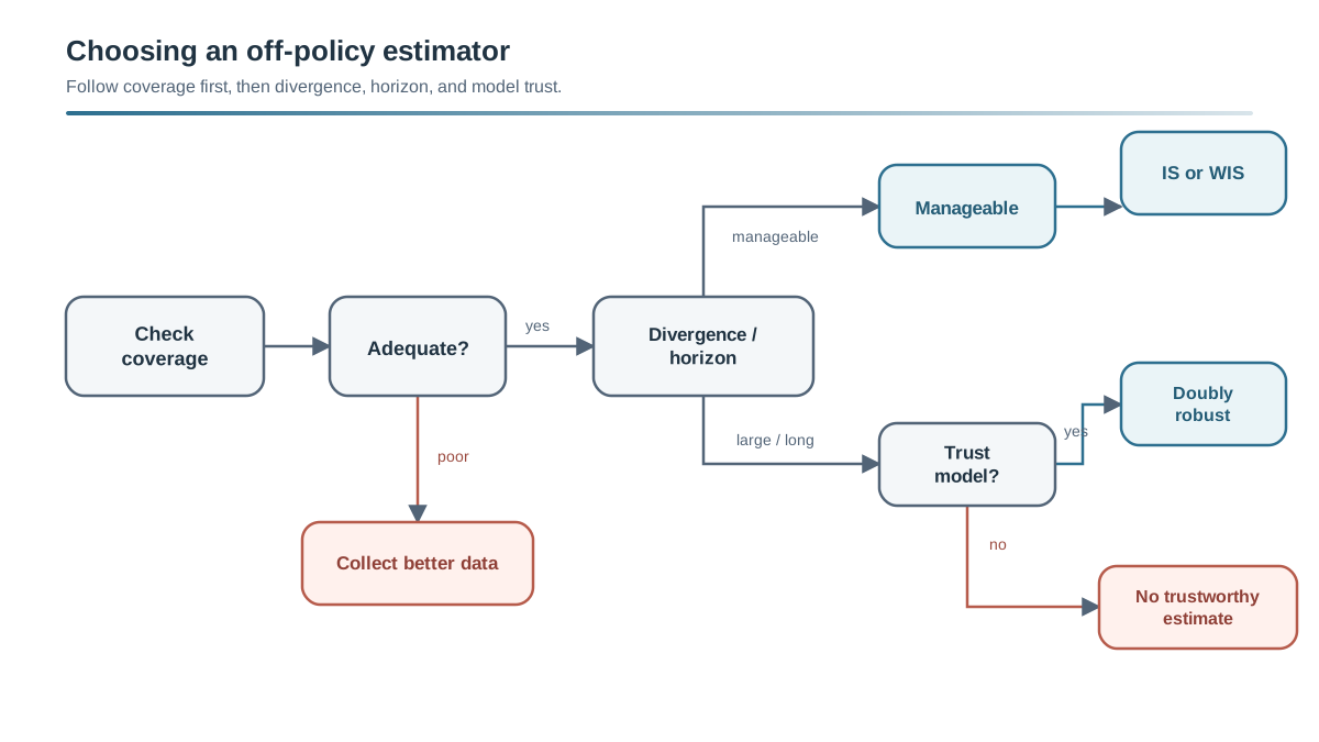
The estimator you choose is a declaration of what you trust. Ordinary importance sampling trusts the logs completely and pays for that trust in variance. Weighted importance sampling trades a little bias for stability. Doubly robust estimation trusts a learned model to buy back variance, and its reliability is bounded by where that model is actually accurate.

Before you compute anything, inspect your dataset. Measure the coverage. Estimate the policy divergence. Look at the horizon length. Then pick the estimator that matches the evidence.

And treat a single point estimate as suspect until you have checked its variance. Resample the trajectories, rerun the estimator across seeds, and look at the spread of the results. If the estimate swings wildly across resamples, the method is telling you something: the logs are thinner than you hoped, the policies are farther apart than you assumed, or the horizon is compounding divergence faster than any correction can contain. The variance is not a nuisance. It is the diagnostic.

References

Research updated Sep 9, 2026