
Derive a Conservative Policy-Improvement Rule From Logged Data
A candidate policy that looks better on paper is not the same as a candidate policy that is better. Here is one small, honest rule for telling the…

Key topics
A candidate policy that looks better on paper is not the same as a candidate policy that is better. Here is one small, honest rule for telling the difference.
You have a fixed dataset. You have a behavior policy that generated it. You have a handful of candidate policies you want to evaluate, and you want to know which one, if any, is worth trusting. The naive answer — pick the candidate with the largest estimated value gain — is exactly the answer that gets you into trouble offline.
This article builds one decision rule: a lower confidence bound on the value gain. It is not a full offline RL algorithm. It is a bounded accept/reject test you can apply to a small set of proposed policy changes, and it is honest about what it cannot do.
Why a Bigger Estimated Gain Is Not a Better Policy Change
The default instinct is reasonable. Estimate the value of each candidate policy from the logged data, subtract the behavior policy's value, and ship whichever candidate has the largest positive gain. When the candidate's actions are well covered by the dataset, this works. The estimate is anchored to real transitions. The number means something.
It breaks when the candidate wants to take actions the behavior policy rarely or never took. Function approximation does not know the difference between "I have evidence this action is good" and "I have no evidence, so I will interpolate optimistically." It fills the gap with a number. That number can be large, and it can be fiction.
If you have already worked through dataset coverage and extrapolation error, you know the mechanism. This article adds a decision layer on top: given that some estimates are trustworthy and some are not, how do you decide? The deliverable is a single criterion, not a training procedure.
Notation and the Finite-Action Setting
Let the state set and action set both be finite. A behavior policy generated the logged dataset . A candidate policy is what we want to evaluate. Define the value of a policy as its expected discounted return:
The quantity we actually care about is the value gain:
We never observe directly. We compute an estimate from , and we attach an uncertainty scale to that estimate. Two assumptions do the real work here:
- Support. The candidate's action distribution must stay inside the region the behavior data covers. If concentrates probability on actions the dataset barely contains, both and stop being meaningful together.
- Calibration. must reflect real estimation error. A number that looks like an error bar but was chosen for convenience is worse than no error bar, because it invites false confidence.
The criterion is defined per candidate change, so you can apply it to a small set of proposed policies and compare.
Knowledge check
Check your understanding
Answer this question before you continue.
Deriving the Penalized Acceptance Rule
Start naive. Accept a candidate if its estimated gain is positive:
This rule treats every estimate as equally trustworthy. It has no way to distinguish a gain of measured tightly from a gain of measured on noise.
Now introduce the penalty. Subtract from the estimate, where controls how skeptical we are:
The acceptance rule becomes: accept only if the lower confidence bound is positive.
Rearrange, and the rule reads more naturally:
The estimated gain must beat its own error bar. That is the whole idea. A big number with a bigger error bar loses to a modest number with a tight one.
is a dial between timid and reckless. At , the penalty vanishes and you are back to the naive rule. As grows, you demand more evidence before accepting a change. The choice of is a risk-tolerance decision, not something the data hands you.
What does the confidence interpretation buy? Under a calibrated , a positive LCB is evidence that the true gain is plausibly positive. It is not proof. The word "confidence" is doing real work, and it depends entirely on the calibration assumption holding.
Knowledge check
Check your understanding
Answer this question before you continue.
A Worked Comparison: Modest Gain, Wide Support vs. Large Gain, Thin Support
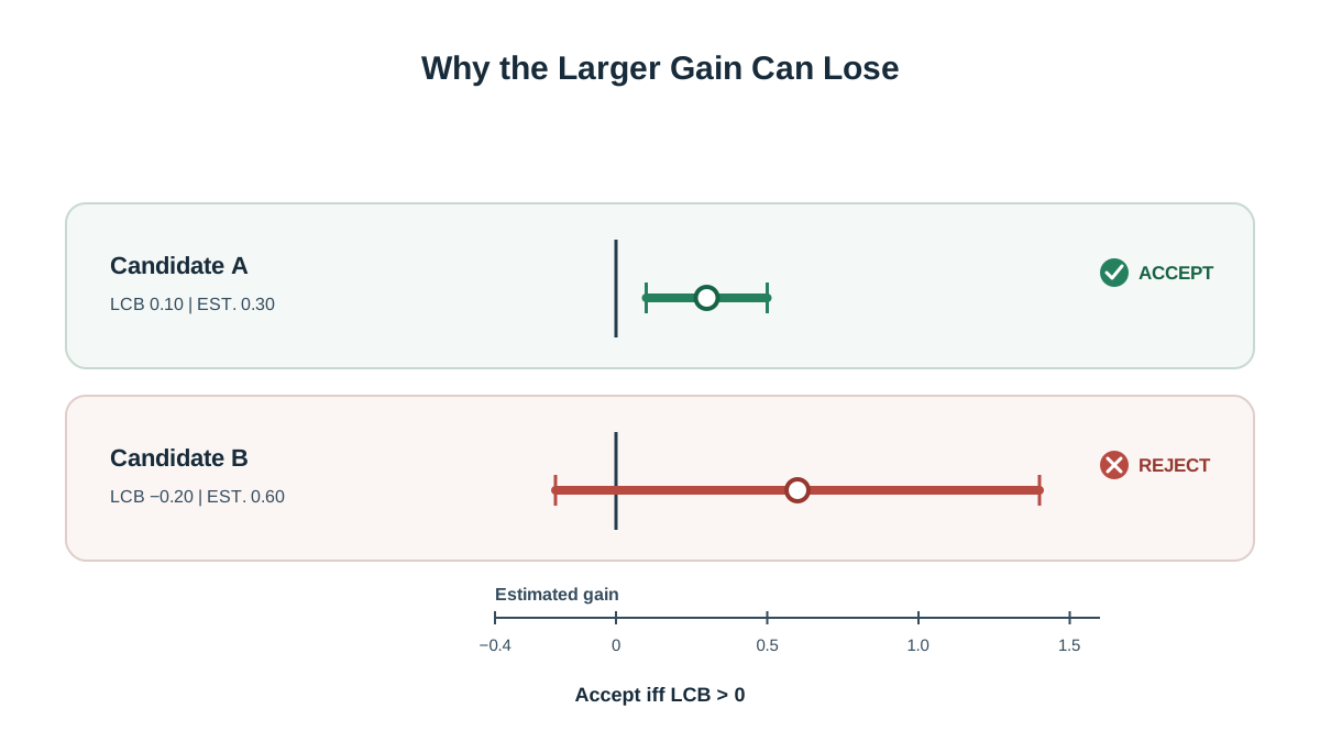
Two candidates, one dataset, .
Candidate A changes an action that appears frequently in the logged data. Its estimated gain is modest, and its uncertainty is small:
Positive. Accept.
Candidate B changes an action the behavior policy rarely took. Its estimated gain is larger, but so is its uncertainty:
Negative. Reject.
Side by side, the reversal is the point:
| Candidate | LCB | Decision | |||
|---|---|---|---|---|---|
| A (well covered) | 0.30 | 0.10 | 2 | 0.10 | Accept |
| B (thin support) | 0.60 | 0.40 | 2 | −0.20 | Reject |
Candidate B has double the estimated gain and still loses, because its error bar is four times wider. The rule is buying evidence, not optimism.
Now vary on the same two candidates. At , and — a tie. Below , B wins; above it, A wins. That flip point is where your skepticism changes the ranking, and it is worth knowing for any pair of candidates you compare.
Picture it as a horizontal axis for with a zero line. Each candidate is a point with an error bar of half-width . A candidate is accepted only if its entire bar sits to the right of zero. Candidate A's bar clears the line. Candidate B's bar straddles it, so the rule refuses to call the gain real.
Knowledge check
Check your understanding
Answer this question before you continue.
What the Rule Assumes, and What Breaks When They Fail
The derivation is short. The assumptions are where the honesty lives.
Calibration failure. If is systematically too small, the penalty is cosmetic. The rule accepts unsupported changes while looking rigorous. This is the most dangerous failure because it is invisible in the output — you get a confident accept from a broken error bar.
Support failure. If the candidate drifts outside behavior-data coverage, and become unreliable together. The penalty cannot rescue an estimate whose foundation is gone. Support is a precondition, not a term in the formula.
Finite-sample noise. With little data, is itself estimated. The bound is only as good as that estimate, and small datasets make the estimate noisy.
Choice of . The data does not supply . You do. Different values produce different decisions on the same candidates, as the flip point above shows.
This is why the rule is illustrative rather than a general safety certificate. It constrains one candidate change under stated assumptions. It says nothing about long-horizon compounding error, and nothing about policies far outside support. Treat it as a disciplined filter, not a guarantee.
Knowledge check
Check your understanding
Answer this question before you continue.
When to Reach for This Rule, and When Not To
Use it when you have a small set of candidate policy changes and need a defensible accept/reject test under limited support. Use it as a sanity check layered on top of a conservative value estimate, not as a replacement for one.
Do not use it as a deployment safety argument. Do not treat a positive LCB as a guarantee of monotonic improvement. Do not skip held-out evaluation because the bound looked clean. And do not apply it to a candidate that sits far outside the behavior distribution — the assumptions are already violated, and the arithmetic will not save you.
The rule earns its keep at the boundary: candidates that are close enough to the data to be estimable, but different enough that you want a reason to trust the change.
Before you accept any offline policy change, ask two questions: what is the error bar, and does the data actually support the action being changed? If you cannot answer both, the estimate is not ready to decide on.
A concrete next move: take two candidate changes from your own logged dataset, compute and for each, and sweep from 0 upward. Record where the decision flips. That flip point tells you how much of your conclusion rests on evidence and how much rests on optimism. The natural next question is where comes from in the first place — which is the job of conservative value estimation, the machinery that produces the uncertainty this rule depends on.
Knowledge check
Final check
Finish the article by checking the ideas you just learned.
References
Build a stronger RL mental model
Use structured resources to connect equations, algorithms, and observable agent behavior.


