Derive Importance Sampling and Doubly Robust Off-Policy Evaluation

You have a log of episodes from one policy, a candidate policy you have never deployed, and a single number that claims to be the candidate's value. The number came from an estimator. The estimator did not run the candidate policy. It reweighted what it saw.

That reweighting is the whole game, and it is only as trustworthy as the overlap between the two policies. This article derives the trajectory importance weight, builds the doubly robust correction on top of it, and then marks the boundary where the derivation stops protecting you.

Setup: Behavior Policy, Target Policy, and What Is Actually Observed

Fix the data-generating process before touching any formula.

The behavior policy $\mu$ generated the logged trajectories. Every action in your dataset was sampled from $\mu(\cdot \mid s_t)$. The target policy $\pi$ is the candidate whose value $J(\pi)$ you want. It never touched the environment. That asymmetry is the entire problem: you have samples from one distribution and a question about another.

Assume a finite horizon $H$, a discounted return with factor $\gamma$, and that you know $\mu$'s action probabilities (or can recover them from the logging system). Define the per-step ratio

$\rho_t = \frac{\pi(a_t \mid s_t)}{\mu(a_t \mid s_t)}$

and the cumulative ratio $\rho_{1:t} = \prod_{t'=1}^{t} \rho_{t'}$.

One precondition does all the heavy lifting later: coverage. Wherever $\pi(a \mid s) > 0$, we need $\mu(a \mid s) > 0$. If the target policy would take an action the behavior policy never takes, the ratio is undefined — you are dividing by zero, and no estimator repairs that. If $\mu$ merely makes that action rare, the ratio is finite but enormous. Zero overlap breaks the math; near-zero overlap breaks the estimate.

If expected values and density rewriting feel shaky, the prerequisite math path covers that ground. Here we assume you accept that an expectation over one distribution can be rewritten by multiplying and dividing by another density.

Why the Trajectory Likelihood Ratio Is a Product of Per-Step Ratios

Write the probability of a trajectory $\tau = (s_1, a_1, \dots, s_H, a_H)$ under a policy. It factors into an initial-state term, a transition term, and an action term:

$P_\pi(\tau) = p(s_1) \prod_{t=1}^{H} P(s_{t+1} \mid s_t, a_t)\, \pi(a_t \mid s_t).$

Now divide the target probability by the behavior probability:

$\frac{P_\pi(\tau)}{P_\mu(\tau)} = \frac{p(s_1) \prod_t P(s_{t+1} \mid s_t, a_t)\, \pi(a_t \mid s_t)}{p(s_1) \prod_t P(s_{t+1} \mid s_t, a_t)\, \mu(a_t \mid s_t)}.$

The initial-state density cancels. The transition density cancels — it does not depend on the policy. What survives is the action probabilities:

$\frac{P_\pi(\tau)}{P_\mu(\tau)} = \prod_{t=1}^{H} \frac{\pi(a_t \mid s_t)}{\mu(a_t \mid s_t)} = \rho_{1:H}.$

The product form is not a rule to memorize. It is what remains after the policy-independent terms cancel. Each step where the target policy was more likely to take the observed action multiplies the weight up. Each step where it was less likely multiplies it down. Over a long horizon, those multiplications compound.

The trajectory-wise estimator applies the full weight to the whole return:

$\hat{V}_{\text{IS}} = \rho_{1:H} \sum_{t=1}^{H} \gamma^{t-1} r_t.$

The step-wise (per-decision) variant applies the prefix weight to each reward separately:

$\hat{V}_{\text{step-IS}} = \sum_{t=1}^{H} \gamma^{t-1} \rho_{1:t}\, r_t.$

Both have the same expectation. The step-wise form has lower variance because a reward collected early is not multiplied by ratios from steps that had not happened yet. That is the version worth defaulting to.

Unbiasedness Under Coverage, and Where the Guarantee Stops

The unbiasedness argument is short. Take the expectation of the weighted return under $\mu$:

$\mathbb{E}_{\mu}\!\left[\rho_{1:H}\, G\right] = \int P_\mu(\tau)\, \frac{P_\pi(\tau)}{P_\mu(\tau)}\, G(\tau)\, d\tau = \int P_\pi(\tau)\, G(\tau)\, d\tau = J(\pi).$

The weight converts one measure into the other. That is the entire proof, and it holds only when the ratio is finite almost surely under $\mu$ — which is exactly the coverage condition. The proof does not merely prefer coverage. It requires it.

Now the part the proof does not promise. The weight is a product of $H$ ratios. Even if each ratio is modest, the product's variance can grow exponentially in the horizon. A weight of $1.2$ per step over twenty steps is a multiplier near $38$. One trajectory can dominate the average.

This is where effective sample size earns its place. If a handful of trajectories carry almost all the weight, your estimate is effectively an average over a handful of samples, no matter how many episodes you logged. The number of episodes is not the number of samples that mattered.

Decision boundary: When the target and behavior policies are close and the horizon is short, plain importance sampling is defensible. When either condition fails, the estimate is dominated by noise, and you should reach for a lower-variance estimator.

The Direct Method and the Residual It Leaves Behind

The direct method fits an approximate value function $\hat{Q}$ or $\hat{V}$ and reads off the target policy's value with no importance weight at all:

$\hat{V}_{\text{DM}} = \mathbb{E}_{s \sim d_\pi}\!\left[\hat{V}(s)\right].$

Its bias comes from model error, and that error is invisible from the data alone. Collecting more episodes does not shrink it — you are converging confidently to the wrong answer.

Define the per-step residual as the observed return minus the model's prediction:

$\delta_t = r_t + \gamma \hat{V}(s_{t+1}) - \hat{Q}(s_t, a_t).$

A good model makes residuals small and roughly centered. A bad model leaves a structured gap. That gap is the raw material the correction will reweight.

The tradeoff is now on the table: the direct method is low variance and biased; importance sampling is unbiased and high variance. The doubly robust estimator is the attempt to keep the good half of each.

Deriving the Doubly Robust Correction

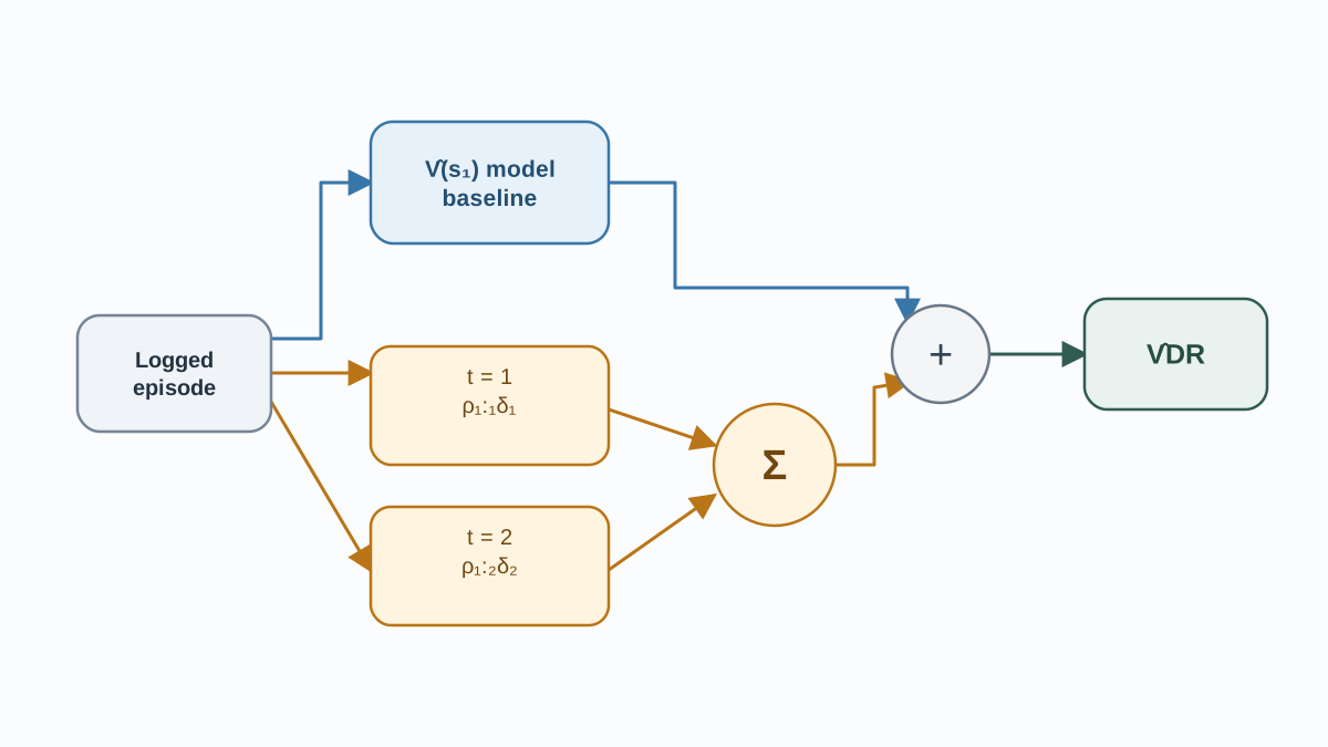
The doubly robust estimator is easiest to read as an episode-level quantity. For a single logged episode, define the direct-method estimate as the model's value at the episode's starting state:

$\hat{V}_{\text{DM}}(\tau) = \hat{V}(s_1).$

This is the model's prediction of the return the target policy would collect from $s_1$. It is a per-episode baseline, not yet an average over the target-policy state distribution. Averaging $\hat{V}(s_1)$ over many episodes drawn from the target policy's initial-state distribution recovers the population-level direct method.

Now add a weighted residual term to that baseline:

$\hat{V}_{\text{DR}}(\tau) = \hat{V}(s_1) + \sum_{t=1}^{H} \gamma^{t-1} \rho_{1:t}\, \delta_t, \qquad \delta_t = r_t + \gamma \hat{V}(s_{t+1}) - \hat{Q}(s_t, a_t).$

The baseline is the model's guess. The sum is the model's correction, weighted by how much the target policy cared about each step. Why does this stay unbiased? Two separate arguments, and you need only one of them.

If the model is correct, then $\mathbb{E}[\delta_t \mid s_t, a_t] = 0$ for every step. The weighted residual term has expectation zero, so the estimator reduces to the direct method — which is already correct. The correction adds nothing but noise, and that noise is centered.

If the model is wrong but the weights are valid, the weighted residual term absorbs the model's error. The direct-method bias is exactly the quantity the residual term estimates and subtracts, because the importance weight makes the residual average over the target policy's distribution rather than the behavior policy's.

That is the doubly robust property stated precisely: unbiased if either the model or the weights are correct — not both. It is a weaker promise than the name suggests. It does not repair zero overlap, and it does not remove variance from the weight itself. If the weights are heavy-tailed, the correction inherits that tail.

Notice the special case: set $\hat{Q} = 0$ and $\hat{V} = 0$. Then $\delta_t = r_t$, and the estimator collapses back to step-wise importance sampling. The doubly robust form is a generalization, not a replacement.

A Small Numerical Example, Worked by Hand

Take a two-step episode, one state per step, two actions $\{a, b\}$, and $\gamma = 1$. The logged trajectory is $a$ then $b$, with rewards $r_1 = 2$ and $r_2 = 3$.

Step	$\pi(a_t \mid s_t)$	$\mu(a_t \mid s_t)$	$\rho_t$	$\rho_{1:t}$
1 ($a$)	0.8	0.5	1.6	1.6
2 ($b$)	0.3	0.6	0.5	0.8

The cumulative weight is $\rho_{1:2} = 1.6 \times 0.5 = 0.8$.

Trajectory-wise IS: $0.8 \times (2 + 3) = 4.0$.

Step-wise IS: $1.6 \times 2 + 0.8 \times 3 = 3.2 + 2.4 = 5.6$.

Now suppose an imperfect value model predicts $\hat{V}(s_1) = 2.5$, $\hat{Q}(s_1, a) = 2.5$, $\hat{Q}(s_2, b) = 2.0$, and $\hat{V}(s_3) = 0$. The episode-level direct-method baseline is the model's value at the starting state: $\hat{V}_{\text{DM}}(\tau) = \hat{V}(s_1) = 2.5$.

The residuals are $\delta_1 = 2 + \hat{V}(s_2) - \hat{Q}(s_1, a)$ and $\delta_2 = 3 + \hat{V}(s_3) - \hat{Q}(s_2, b)$. Using $\hat{V}(s_2) = 2.0$ and $\hat{V}(s_3) = 0$: $\delta_1 = 2 + 2.0 - 2.5 = 1.5$ and $\delta_2 = 3 + 0 - 2.0 = 1.0$.

Doubly robust: $\hat{V}_{\text{DR}}(\tau) = 2.5 + (1.6 \times 1.5 + 0.8 \times 1.0) = 2.5 + (2.4 + 0.8) = 2.5 + 3.2 = 5.7$.

Three numbers — $4.0$, $5.6$, $5.7$ — from one trajectory. They disagree because they weight the same data differently, and the model's error is large enough that the correction moves the estimate a lot. One trajectory proves nothing statistically. The example shows the mechanics, not a ranking. Do not read a winner out of a single sample.

Support, Variance, and When Not to Trust the Number

Two conditions must hold for any of this to mean anything. First, coverage: the behavior policy must assign positive probability to every action the target policy might take. Second, weights must not be dominated by a few trajectories.

The diagnostics worth computing before you report a value:

• The maximum weight and its distribution. A single weight orders of magnitude above the rest is a warning, not a win.
• Effective sample size, the inverse of the sum of squared normalized weights. It tells you how many trajectories actually carried the estimate.
• A side-by-side comparison against the direct method. If the two disagree wildly, the weights are doing something you should inspect before trusting either.

A high estimated value with heavy-tailed weights is a red flag. It usually means a few trajectories are standing in for the whole target policy, and the estimate is closer to a lottery ticket than a measurement. This is the same coverage boundary that makes offline learning hard — unsupported actions produce unreliable targets whether you are learning or evaluating.

Decision boundary: Use plain importance sampling for short horizons and similar policies. Use a doubly robust form when you have a reasonable model and moderate overlap. Treat any estimate as unusable when overlap is near zero, regardless of which estimator you pick.

These are estimators with sampling error, not guarantees. A point estimate without a variance or interval is an incomplete result.

The Habit That Follows From the Derivation

Before you report any off-policy value, do three things: check overlap, inspect the weight distribution, and report the estimate with its uncertainty rather than as a single number. The derivation tells you why the number is unbiased under coverage. It does not tell you whether your data satisfies the condition.

Your next step is concrete: take your own logged episodes, compute the per-step ratios, and plot the weight distribution and effective sample size. Then run the importance sampling and doubly robust estimates side by side and look at the gap. If the gap is small and the weights are tame, you have a defensible estimate. If the gap is large or the weights are heavy-tailed, you have found the boundary of what your data can support — and that is more valuable than a confident number.