Test How Demonstrations Shape Later Online Reinforcement Learning

A policy cloned from demonstrations can look brilliant and still be useless. It scores well on the states it was shown, then stalls the moment the world drifts off the demonstrated path. The cheapest way to find out whether environment feedback fixes that — or whether the demonstrations quietly cap it — is to run the experiment yourself.

This tutorial builds a small sequential task, freezes a demonstrations-only baseline, trains a learner from scratch, and then trains a learner that starts from the same demonstrations while continuing to receive environment feedback. The decisive number is not "does the learner beat random." It is does the learner beat the frozen demonstration policy.

If you have already written a tabular Q-learning loop and you understand that demonstrations can initialize, guide, or constrain a policy, you have everything you need. We will not re-teach either one here.

What This Experiment Actually Tests

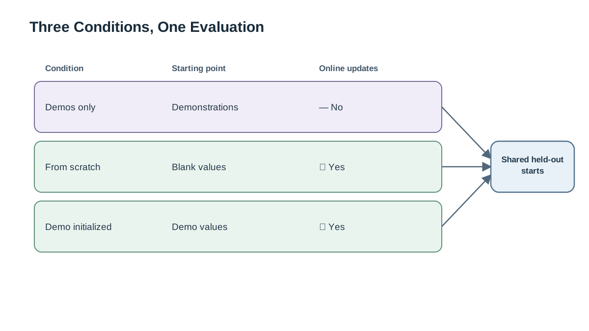
One question: do demonstrations raise the ceiling, or do they become the ceiling?

To answer it, you compare three conditions against a fixed evaluation protocol:

Condition	What it gets	What it can do
Demonstrations-only baseline	The demonstration set	Nothing — the policy is frozen
From-scratch learner	Environment feedback only	Act, update, explore
Demonstration-initialized learner	The same demonstrations plus environment feedback	Start from demonstrated values, then keep updating

The measured quantity is return per episode over training, plus a final evaluation on a held-out set of start states. That second measurement matters more than the first. A policy can look strong on the training distribution and fall apart off it.

State the hypothesis before you write a line of code: feedback should allow improvement beyond the demonstrations only if the demonstrations are suboptimal and the learner can still explore. If either condition fails, expect a flat curve — and expect that flatness to be informative rather than broken.

Prerequisites and Environment Assumptions

You need Python 3, NumPy, and Matplotlib. No deep-learning framework, no GPU, no external services, no credentials.

The task is a small deterministic gridworld with a sparse goal reward and a step penalty. It is small enough that a Q-table is exact and the whole run finishes in seconds.

Why tabular? Because it removes function-approximation noise from the comparison. If a neural network is unstable, you cannot tell whether a difference between conditions came from the demonstrations or from the optimizer. Here, any difference is attributable to the demonstrations.

Fix your seeds and fix your evaluation protocol. Same seeds, same number of evaluation episodes, same starting states for every condition. Without that discipline, you are comparing noise to noise.

Build the Task and the Demonstration Set

Start with the environment. A grid with a goal cell, a step penalty, and termination on reaching the goal is enough:

import numpy as np

GRID = 6
GOAL = (5, 5)
ACTIONS = [(-1, 0), (1, 0), (0, -1), (0, 1)]  # up, down, left, right

def step(state, action):
    r, c = state
    dr, dc = ACTIONS[action]
    nr, nc = min(max(r + dr, 0), GRID - 1), min(max(c + dc, 0), GRID - 1)
    next_state = (nr, nc)
    if next_state == GOAL:
        return next_state, 1.0, True
    return next_state, -0.01, False

Now generate demonstrations from a deliberately imperfect scripted policy. A shortest-path walker with a fixed error rate is ideal: good enough to be useful, bad enough that improvement is possible.

def scripted_action(state, rng, error_rate=0.2):
    if rng.random() < error_rate:
        return int(rng.integers(len(ACTIONS)))
    r, c = state
    gr, gc = GOAL
    if r < gr:
        return 1
    if c < gc:
        return 3
    return 0

def collect_demos(n_episodes, rng):
    demos = []
    for _ in range(n_episodes):
        state, traj = (0, 0), []
        for _ in range(100):
            action = scripted_action(state, rng)
            next_state, reward, done = step(state, action)
            traj.append((state, action))
            state = next_state
            if done:
                break
        demos.append(traj)
    return demos

Record demonstrations both as (state, action) pairs and as full trajectories. The pair list is what you will clone from; the trajectory structure is what you will need later when you reason about credit assignment.

Print the grid, the demonstration success rate, and the average return of the demonstration policy. Those three numbers are your first milestone.

Common mistake: collecting demonstrations that cover only the optimal corridor. If every demo hugs the same path, the covariate-shift failure stays invisible, and you will conclude demonstrations are harmless when you have simply never tested them off-path.

Baseline 1: Freeze the Demonstrations

Fit a simple state-to-action policy from the demonstration pairs. A lookup table with a fallback for unseen states is enough:

def fit_policy(demos):
    counts = {}
    for traj in demos:
        for state, action in traj:
            counts.setdefault(state, np.zeros(len(ACTIONS)))
            counts[state][action] += 1
    return {s: int(np.argmax(v)) for s, v in counts.items()}

def frozen_action(policy, state):
    return policy.get(state, 0)  # fallback: always "up"

Evaluate it on the same protocol you will use for the learner. Report mean return and success rate.

Then watch it break. On states the demonstrations never visited, the fallback action produces a visible stall or a loop — the agent walks into a wall, or oscillates between two cells, forever. That is covariate shift made physical.

Write this number down before you train anything else. It is the comparison baseline the learner must beat.

A high demonstration score is not evidence of a good policy. It is evidence of good coverage. Those are different claims, and conflating them is how people ship imitation policies that fail in production.

Baseline 2: Learn From Scratch

Run a standard tabular Q-learning loop with no demonstrations at all. Same seeds, same evaluation protocol.

def train_q(episodes, rng, lr=0.1, gamma=0.95,
            eps_start=1.0, eps_end=0.05, eps_decay=0.995,
            init_Q=None):
    Q = np.zeros((GRID, GRID, len(ACTIONS))) if init_Q is None else init_Q.copy()
    returns = []
    eps = eps_start
    for _ in range(episodes):
        state, total = (0, 0), 0.0
        for _ in range(100):
            if rng.random() < eps:
                action = int(rng.integers(len(ACTIONS)))
            else:
                action = int(np.argmax(Q[state[0], state[1]]))
            next_state, reward, done = step(state, action)
            best_next = 0.0 if done else np.max(Q[next_state[0], next_state[1]])
            Q[state[0], state[1], action] += lr * (
                reward + gamma * best_next - Q[state[0], state[1], action]
            )
            state, total = next_state, total + reward
            if done:
                break
        returns.append(total)
        eps = max(eps_end, eps * eps_decay)
    return Q, returns

Expect slow early progress. With a sparse goal reward and a step penalty, random exploration rarely reaches the goal, so the value signal arrives late and thin.

This curve answers a different question than the demonstration baseline: how much of the learner's speed comes from the demonstrations versus from the task itself?

Common mistake: comparing the demonstration-initialized learner only against the frozen baseline and concluding demonstrations helped — when the from-scratch learner would have reached the same return anyway, just later. Without this second baseline, you cannot separate "demonstrations accelerated learning" from "the task was easy."

Add Demonstrations to the Learner

Now the actual experimental condition. Initialize the Q-table from the demonstrations — set demonstrated action values above the alternatives:

Q_init = np.zeros((GRID, GRID, len(ACTIONS)))
for traj in demos:
    for state, action in traj:
        Q_init[state[0], state[1], action] = 1.0

Q_demo, returns_demo = train_q(EPISODES, rng, init_Q=Q_init)

That is initialization only: the demonstrated values set the starting point, and after that the standard update loop is free to overwrite them. This is the mechanism the headline three-condition experiment isolates. Guidance — a bonus that keeps pulling the policy back toward demonstrated actions during training — is a separate mechanism, and mixing it in here would make the curve impossible to attribute. We will test it as a follow-up instead.

Evaluate on Held-Out Start States

Training return tells you how the learner behaves on the distribution it trained on. It does not tell you whether the policy generalizes. Define a fixed held-out set of start states and evaluate every condition on the same starts:

EVAL_STARTS = [(0, 0), (0, 3), (2, 2), (3, 0), (4, 4)]

def evaluate(Q, starts, rng, episodes_per_start=20):
    scores = []
    for start in starts:
        for _ in range(episodes_per_start):
            state, total = start, 0.0
            for _ in range(100):
                action = int(np.argmax(Q[state[0], state[1]]))
                state, reward, done = step(state, action)
                total += reward
                if done:
                    break
            scores.append(total)
    return float(np.mean(scores))

For the frozen policy, replace the argmax line with frozen_action(policy, state). For the from-scratch learner, pass its Q. For the demonstration-initialized learner, pass Q_demo.

Now plot all three curves on one axis:

import matplotlib.pyplot as plt

plt.plot(returns_frozen, label="demonstrations only")
plt.plot(returns_scratch, label="from scratch")
plt.plot(returns_demo, label="demo-initialized")
plt.xlabel("episode")
plt.ylabel("return")
plt.legend()
plt.show()

Expected output: the frozen baseline is a flat horizontal line. The from-scratch curve climbs slowly. The demo-initialized curve starts high and either keeps climbing or flattens below the frozen line. Both outcomes are results.

Read the Curves: Did Feedback Beat the Demonstrations?

The interesting outcome is a learner that starts near the demonstration return and then exceeds it. That is feedback doing work the demonstrations could not.

The disappointing outcome is a learner that starts high and stays flat or decays. Diagnose the cause before you blame the method:

• Too little exploration — epsilon decayed too fast, so the learner never found states the demonstrations missed.
• Demonstrations that already saturate the task — there is simply no headroom left.
• Initial values too confident for the update rule to correct within the episode budget.

Report the held-out evaluation separately from training return. A policy can look strong on the training distribution and fail off it, and that gap is often the most important number in the whole run.

Decision rule: if the learner never exceeds the frozen baseline, the demonstrations are acting as a ceiling, not a springboard.

Failure Modes and Debugging Signals

Symptom	Likely cause	One change to try
Flat curve at the demonstration level	Exploration collapsed	Raise the epsilon floor; slow the decay
Curve drops after initialization	Initial values too confident for the update rule to correct, or learning rate too high for pre-filled values	Lower the learning rate; reduce the initial value magnitude
Strong training return, weak held-out return	Policy memorized demonstration states and never generalized	Evaluate on the held-out starts; add exploration
Noisy, non-monotonic curve	Too few episodes or a single seed	Average over several seeds before drawing conclusions

Each symptom maps to one concrete change. Make it, re-run, and compare against the original three curves on the same axes.

One Modification Worth Running

Change one variable at a time. Pick one:

• Demonstration quality — raise the scripted policy's error rate.
• Demonstration quantity — collect fewer trajectories.
• Guidance — add a decaying bonus for demonstrated actions and compare it against initialization-only.

Predict the outcome before you run it. My expectation: noisier demonstrations should lower the starting return but may raise the final return, because feedback has more room to correct them. If that prediction holds, you have learned something about the mechanism, not just about the code.

Compare the modified run against the original three curves. This is where you find out whether demonstrations are a starting point or a constraint in your setup, not just in this article's.

What the Experiment Earns You

Demonstrations buy you a starting point. Environment feedback is what buys you a ceiling above it. If the learner never passes the frozen baseline, the demonstrations are constraining rather than accelerating — and now you have the curve to prove it.

The natural next step is to vary demonstration quality and quantity systematically, then read the results as evidence about your own pipeline rather than as a leaderboard. The question is never "are demonstrations good?" It is "good for what, and at what cost to the learner's freedom to improve?"