
Compare Greedy and Exploratory Strategies in a Contextual Bandit With Python
A greedy agent looks brilliant for the first fifty rounds. Then it stops learning, because it stopped asking questions.

Key topics
A greedy agent looks brilliant for the first fifty rounds. Then it stops learning, because it stopped asking questions.
That is the whole experiment in one sentence. We are going to build a small world where the best action depends on the situation, run two decision rules against it, and watch one of them quietly stall. No state transitions, no neural networks, no GPU. Just numpy, matplotlib, and a question worth answering: does exploration actually pay for itself?
If you have read the intuition pieces on contextual bandits and the exploration-exploitation tradeoff, this is where that mental model becomes a number you can print. If you have not, the short version is enough to start: a contextual bandit is a one-step decision problem. The world shows you a context, you pick one action, you get one reward, and tomorrow's context does not care what you chose today.
What We Are Building and Why It Is Small on Purpose
The setting is a stationary contextual bandit. Each round, the world generates a context vector. The agent picks one of a fixed set of arms. Only the chosen arm's reward is revealed — the rest stay hidden, which is exactly why this is hard.
Stationary means the hidden reward rules never change. That is a deliberate simplification. If the rules drifted over time, we could not tell whether a strategy was learning or just chasing noise.
No state transitions means today's action does not shape tomorrow's context. That is the boundary between this and full reinforcement learning, and it is why we can measure regret cleanly: every round is an independent chance to be right or wrong.
Two numbers carry the whole comparison:
- Cumulative reward — the total collected so far. Higher is better.
- Cumulative regret — the gap between what we earned and what a clairvoyant policy would have earned by always picking the best arm for each context. Lower is better.
Regret is the honest metric. Reward can look fine while you are leaving a lot on the table; regret tells you how much.
Assumptions before we start: Python 3, numpy and matplotlib installed, no credentials, no external services, no GPU. If pip install numpy matplotlib works, you are ready.
Designing the Simulated World
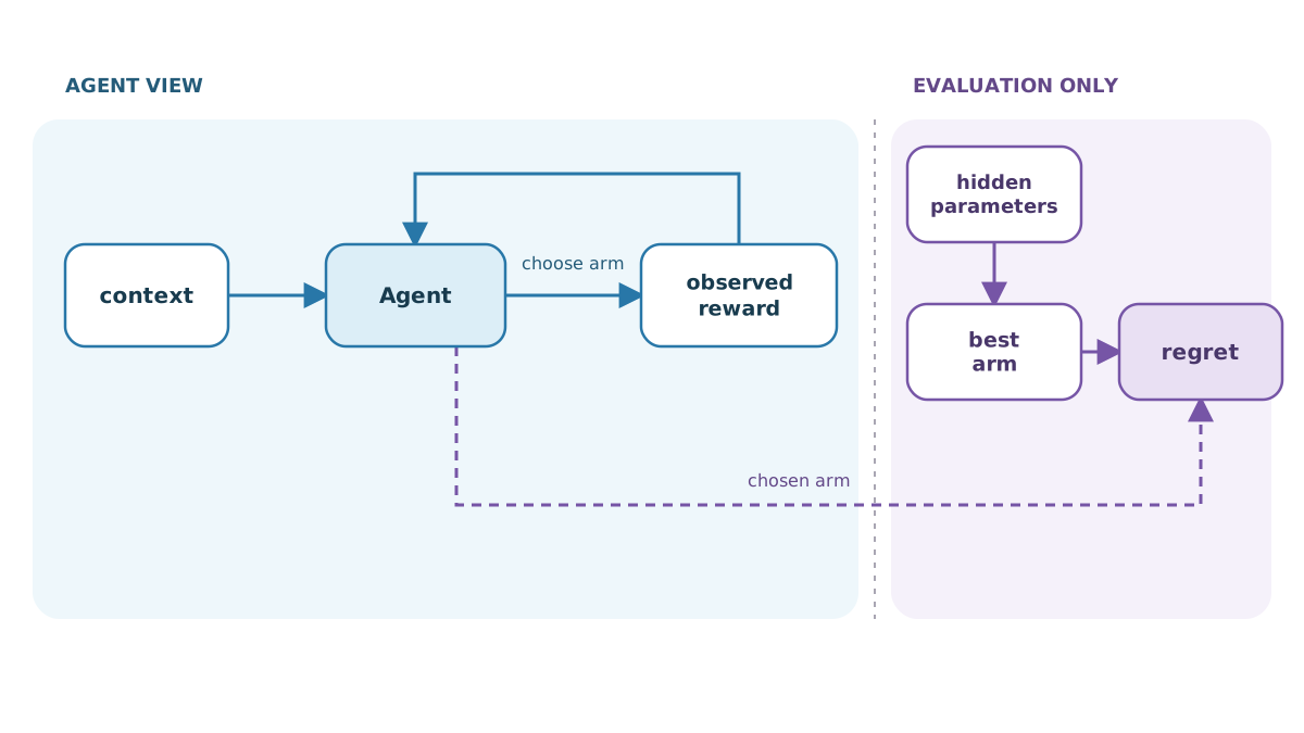
Build the answer key before the agent starts guessing. That is the only way to know whether the agent is doing well.
We will use a logistic reward model: each arm has a hidden parameter vector, and the probability of reward depends on the dot product between the context and that vector. This matters because the best arm genuinely changes with the context. A fixed best arm would make this a plain multi-armed bandit wearing a costume.
import numpy as np

N_ARMS = 3
N_FEATURES = 4

def make_world(seed=0):
    rng = np.random.default_rng(seed)
    # Hidden per-arm parameters the agent never sees
    theta = rng.normal(size=(N_ARMS, N_FEATURES))
    return theta, rng

def sample_context(rng):
    return rng.normal(size=N_FEATURES)

def true_prob(context, arm, theta):
    z = context @ theta[arm]
    return 1.0 / (1.0 + np.exp(-z))

def step(context, arm, theta, rng):
    p = true_prob(context, arm, theta)
    return 1 if rng.random() < p else 0

def best_arm(context, theta):
    # Evaluation only. The agent must never call this.
    probs = [true_prob(context, a, theta) for a in range(N_ARMS)]
    return int(np.argmax(probs))
The agent sees context and arm. It does not see theta. That separation is the entire learning problem: the agent has to infer the hidden parameters from noisy one-bit feedback, one arm at a time.
Before adding any policy, confirm the world works:
theta, rng = make_world(seed=1)
for _ in range(5):
    ctx = sample_context(rng)
    arm = rng.integers(N_ARMS)
    r = step(ctx, arm, theta, rng)
    print(f"context={np.round(ctx, 2)} arm={arm} reward={r}")
You should see five lines, each with a context vector, a chosen arm, and a 0 or 1. If that prints, the world is alive. Now we can start guessing.
Knowledge check
Check your understanding
Answer this question before you continue.
A Greedy Baseline: Commit Early, Pay Later
The simplest policy estimates each arm's value with a running average of observed rewards and always picks the highest estimate.
def run_greedy(theta, rng, rounds=2000):
    counts = np.zeros(N_ARMS)
    sums = np.zeros(N_ARMS)
    rewards, regrets = [], []

    for _ in range(rounds):
        ctx = sample_context(rng)
        # Untried arms get priority so estimates exist at all
        if np.any(counts == 0):
            arm = int(np.argmin(counts))
        else:
            arm = int(np.argmax(sums / counts))

        r = step(ctx, arm, theta, rng)
        counts[arm] += 1
        sums[arm] += r

        rewards.append(r)
        regrets.append(true_prob(ctx, best_arm(ctx, theta), theta)
                      - true_prob(ctx, arm, theta))

    return np.cumsum(rewards), np.cumsum(regrets)
Run it and look at the regret curve. You should see a fast start and then a flattening — the agent stops improving because it stops gathering evidence. An arm that got lucky on its first sample becomes permanently "best," and the agent never revisits the alternatives.
Common mistake: assuming a flat reward curve means the agent has converged on the right answer. It usually means the agent has converged on an answer and stopped checking.
The diagnostic signal is regret that grows roughly linearly instead of leveling off. Linear regret means you are paying the same mistake over and over.
Knowledge check
Check your understanding
Answer this question before you continue.
Adding Epsilon-Greedy Exploration
Here is the entire change: with probability epsilon, pick a uniformly random arm. Otherwise, pick the greedy arm.
def run_epsilon_greedy(theta, rng, rounds=2000, epsilon=0.1):
    counts = np.zeros(N_ARMS)
    sums = np.zeros(N_ARMS)
    rewards, regrets = [], []

    for _ in range(rounds):
        ctx = sample_context(rng)
        if rng.random() < epsilon or np.any(counts == 0):
            arm = int(rng.integers(N_ARMS))
        else:
            arm = int(np.argmax(sums / counts))

        r = step(ctx, arm, theta, rng)
        counts[arm] += 1
        sums[arm] += r

        rewards.append(r)
        regrets.append(true_prob(ctx, best_arm(ctx, theta), theta)
                      - true_prob(ctx, arm, theta))

    return np.cumsum(rewards), np.cumsum(regrets)
Notice what did not change: the world, the estimator, the reward model. Only the action-selection rule moved. That is the point of a controlled experiment — one variable at a time.
Two regimes matter here. A fixed epsilon keeps paying a permanent exploration tax: you keep spending 10% of your rounds on random arms forever. A decaying epsilon spends early rounds buying information and later rounds cashing it in. Both are legitimate; they just trade off differently.
The honest limitation: epsilon-greedy explores blindly. It cannot tell a promising-but-uncertain arm from one it already knows is bad. It rolls the dice the same way regardless.
Knowledge check
Check your understanding
Answer this question before you continue.
Running the Comparison Across Many Seeds
One run proves nothing. A single lucky seed can make a bad policy look brilliant, and a single unlucky one can bury a good policy. Averaging over many runs is the minimum bar for any claim.
def average_over_seeds(runner, seeds=range(30), rounds=2000, **kwargs):
    all_rewards, all_regrets = [], []
    for s in seeds:
        theta, rng = make_world(seed=s)
        r, g = runner(theta, rng, rounds=rounds, **kwargs)
        all_rewards.append(r)
        all_regrets.append(g)
    return np.mean(all_rewards, axis=0), np.mean(all_regrets, axis=0)

greedy_r, greedy_g = average_over_seeds(run_greedy)
eps_r, eps_g = average_over_seeds(run_epsilon_greedy, epsilon=0.1)
Plot both policies on the same axes:
import matplotlib.pyplot as plt

plt.plot(greedy_g, label="greedy")
plt.plot(eps_g, label="epsilon-greedy (0.1)")
plt.xlabel("round")
plt.ylabel("mean cumulative regret")
plt.legend()
plt.show()
What you should see: the exploratory policy ends with lower average regret over the horizon, and the gap widens rather than closes. Early rounds may favor greedy — that is expected, not a bug. Greedy cashes in immediately; epsilon-greedy pays a small tax up front to learn which arm is actually best.
| Greedy | Epsilon-greedy | |
|---|---|---|
| Early rounds | Fast reward, low regret | Slightly worse (exploration tax) |
| Late rounds | Regret grows linearly | Regret grows more slowly, but still grows |
| Exploration | None after initial pass | Continuous or decaying |
| Failure mode | Locks onto a lucky arm | Never settles if epsilon is too high |
If the two curves are indistinguishable, do not blame the algorithm yet. Check the exploration rate and the estimator first.
Knowledge check
Check your understanding
Answer this question before you continue.
When the Numbers Disagree With Your Intuition
Real experiments break in predictable ways. Here are the ones I see most often.
Epsilon too high. The agent never settles. Regret stays linear and the curve looks like pure noise. You are exploring more than you are learning.
Epsilon too low. The agent behaves like the greedy baseline and the two curves overlap. That overlap is a signal that you are not actually testing exploration.
Reward scale or sign errors. If rewards are all negative or wildly scaled, running averages mislead and the comparison becomes meaningless. Keep rewards bounded and consistent.
Forgetting to seed, or reusing one seed for both policies. The comparison becomes unfair or irreproducible. Give each policy the same seed set so they face the same world.
Context leakage. If the agent can see best_arm, the experiment becomes a lookup table and the real learning problem disappears. Keep the answer key out of the agent's reach.
Tip: If the two curves are indistinguishable, suspect the exploration rate or the estimator before suspecting the algorithm. The mechanism is usually fine; the knobs are wrong.
One Modification Worth Trying Next
The greedy and epsilon-greedy agents above are context-blind: they average rewards per arm across all contexts. That works here only because the world is simple. Make the estimator context-aware — fit a small per-arm logistic regression on the context — and predict what should happen before you run it.
A context-aware policy should beat a context-blind one when the best arm genuinely depends on the context. Then test the boundary: shrink the context's influence on rewards and watch the advantage disappear. That is how you learn the method is not magic — it is a fit to a structure that may or may not exist.
A cheaper variation: sweep epsilon over a few values and plot final regret against epsilon. You get the tradeoff as a curve instead of a guess.
Once one-step credit assignment feels concrete, the natural next step is sequential state transitions and temporal-difference learning, where today's action does shape tomorrow's situation. Same simulator instincts, harder problem.
Greedy is a measurement, not a strategy. It tells you what your current estimates believe — and it stops telling you anything the moment it stops exploring. Run the experiment. Watch the curves separate. Then change one thing and watch them separate differently.
Knowledge check
Final check
Finish the article by checking the ideas you just learned.
References
Build a stronger RL mental model
Use structured resources to connect equations, algorithms, and observable agent behavior.


