A Small Tabular RL Experiment: Watch Exploration Become a Policy

A Q-table makes the invisible visible. Before neural networks, before GPUs, before thousands of parameters, there is a simple grid, a handful of numbers, and the exact moment random wandering becomes deliberate navigation.

Why Start With a Table Instead of a Neural Network

The core loop of reinforcement learning is small: the agent observes a state, picks an action, receives a reward, and updates what it knows. That loop is identical whether the learner is a lookup table or a deep neural network. The only difference is where the knowledge lives.

A Q-table stores one number for every state-action pair. If your environment has 16 states and 4 actions, that is 64 numbers. You can print all of them. You can watch them change after every episode. When the agent makes a mistake, you can point at the exact value that caused it.

A neural network does the same job with function approximation. It generalizes across states it has never seen, which is powerful—and also opaque. If you cannot read a Q-table, a network will hide the mechanism you are trying to learn behind thousands of parameters.

This experiment teaches you three things: how exploration discovers useful experience, how a single update step turns that experience into knowledge, and how to read a learning curve like a diagnostic tool. It will not teach you scaling or generalization. That comes later, and it will be easier because you built the foundation first.

The Tiny Environment: One Goal, One Trap, One Grid

Imagine a 4x4 grid. The agent starts in the top-left corner. The goal sits in the bottom-right corner. Somewhere in between, there is a trap.

S  .  .  .
.  .  T  .
.  .  .  .
.  .  .  G

The agent can move up, down, left, or right. Hitting the trap ends the episode with a heavy penalty. Reaching the goal ends it with a large reward. Every other step costs a small penalty, which pushes the agent toward shorter paths.

Why this environment? It has a clear optimal path, a tempting wrong path, and enough steps that the agent must learn to connect distant outcomes to earlier decisions. The state space is small enough that the entire Q-table fits on your screen.

The reward design matters. The step penalty makes the agent prefer efficiency. The goal reward makes the destination worth pursuing. The trap penalty makes danger worth avoiding. If any of these numbers are off, the agent will learn something different—sometimes something surprisingly reasonable given what the numbers say.

The Agent's Two Jobs: Explore, Then Exploit

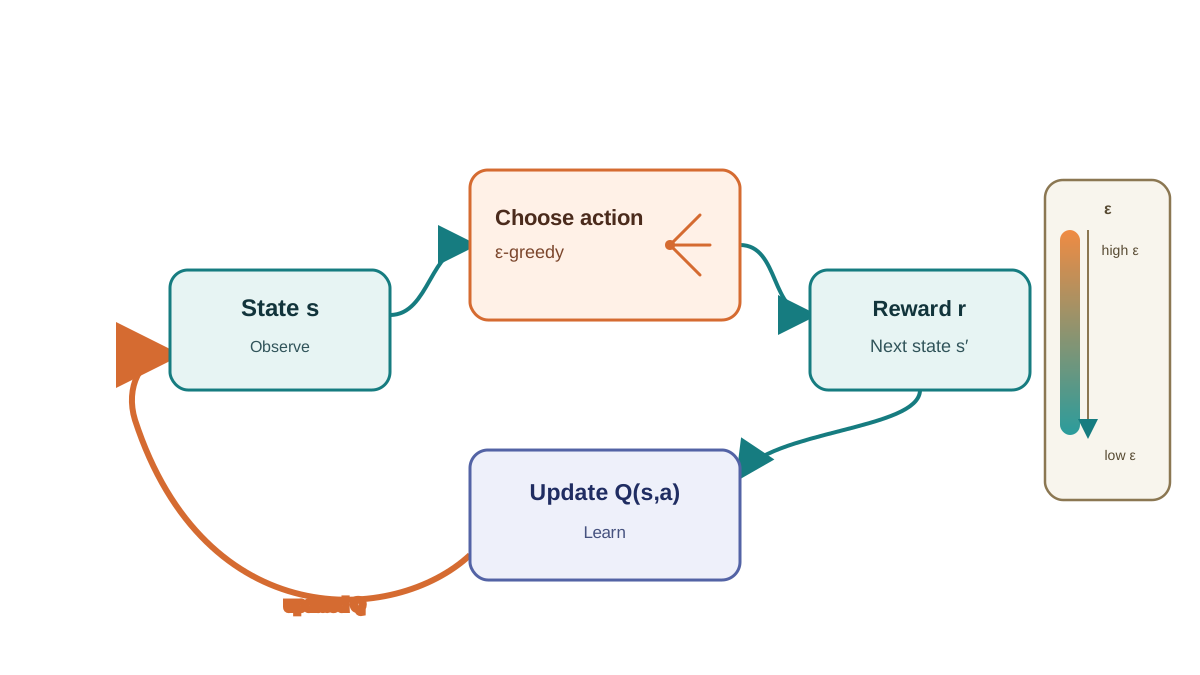
Before running the experiment, you need one mental model: the agent has two conflicting jobs. It must try actions it has not tried before to discover what works. It must also use what it already knows to collect reward. These jobs pull in opposite directions.

The standard solution is called epsilon-greedy. With probability epsilon, the agent picks a random action. Otherwise, it picks the action with the highest Q-value. Epsilon starts high—say 0.9—so early episodes are mostly random wandering. Over time, epsilon decays toward a small floor, and the agent shifts from explorer to exploiter.

The Q-table starts as zeros. That means the "best" action early on is a guess, because every action looks equally good. The agent must explore to break the tie. This is the part beginners often miss: exploration is not a bug in the learning process. It is the engine that generates the data the agent learns from.

In the first episodes, expect to see wandering, collisions with the trap, and the occasional lucky reach of the goal. That noise is not failure. It is the agent collecting information.

The Update Rule: Learning From One Step, Not the Whole Episode

Here is where temporal-difference learning earns its name. The agent does not wait until the episode ends to learn. After every single step, it makes a small update based on what just happened.

The plain-language version of the Q-learning update is this: the new estimate for a state-action pair moves a little toward the reward just received plus the agent's best guess about the value of the next state.

The formula looks intimidating at first, but each piece has a job:

Q(s, a) ← Q(s, a) + α [ r + γ max(Q(s', a')) - Q(s, a) ]

The learning rate alpha controls how much the new experience moves the old estimate. A high alpha means the agent trusts each new step heavily. A low alpha means it updates cautiously.

The discount factor gamma controls how much the agent values future rewards. A gamma near 1 means distant rewards matter almost as much as immediate ones. A low gamma makes the agent myopic, caring mostly about what happens right now.

Walk through one update by hand. Suppose the agent is in a state next to the goal, takes a step, and receives a reward of +10. The old Q-value for that state-action pair is 0. With alpha at 0.1 and gamma at 0.9, the update moves the value from 0 to 1. That single step contains a signal. Repeat it across many episodes, and the value creeps toward its true estimate.

This is the temporal-difference idea in action: the agent learns from a guess about the future, not from the final outcome of the episode. It can learn after every step, which makes it far more sample-efficient than waiting for the end.

Run It: What the Learning Curves Actually Tell You

When you run the experiment, log two things: the total reward per episode and, at intervals, a snapshot of the Q-table or the greedy policy derived from it.

The reward curve tells the story of learning. Early episodes bounce around wildly because exploration injects randomness. Then the curve climbs as the agent starts finding the goal more often. Finally it plateaus, with occasional dips that correspond to exploratory actions.

The curve will be jagged, not smooth. That jaggedness is not a bug. Even late in training, epsilon keeps injecting random actions. The agent occasionally steps into the trap because it is still exploring. The plateau represents the best performance the agent can sustain while maintaining a small amount of curiosity.

The Q-table tells a deeper story. Early on, most values sit near zero because most state-action pairs have never been visited. As training progresses, values near the goal rise first. The signal propagates backward, state by state, like knowledge spreading from the reward outward.

The aha moment comes when you derive the greedy policy from the table: at each state, pick the action with the highest Q-value. If learning worked, that policy should trace the intuitive optimal path from start to goal, avoiding the trap. You are watching exploration become a policy.

When Learning Goes Wrong: Three Failure Cases to Diagnose

Learning curves are diagnostic tools. When the agent fails, the curve tells you why. Here are three failure cases worth running deliberately.

Failure 1: Epsilon never decays. If epsilon stays high, the agent keeps exploring forever and never settles into a reliable policy. The reward curve stays noisy, never climbing to a stable plateau. The fix is to decay epsilon over episodes. The lesson: exploration is only useful when it eventually gives way to exploitation.

Failure 2: Learning rate too high or too low. With a high alpha, Q-values thrash. Each new experience overwrites most of what the agent knew, so the curve bounces violently. With a low alpha, Q-values barely move from their starting guesses, and learning crawls. The fix is to find a middle ground. The lesson: the learning rate controls how much the agent trusts new experience over accumulated knowledge.

Failure 3: Trap penalty too small. If the trap penalty is only slightly worse than the step penalty, the agent may learn a path that clips the trap. The numbers say it is fine: a path that occasionally hits the trap can still beat a longer safe path. The fix is to make the trap penalty severe enough that the optimal policy avoids it. The lesson: reward design shapes behavior, and the agent will exploit any loophole you leave in the numbers.

Change one hyperparameter, rerun, and read the difference. That is the whole drill. Each failure teaches you something about the mechanism that a successful run cannot.

What This Experiment Prepares You For

The same update rule and exploration loop carry over to deep reinforcement learning. Only the function approximator changes: instead of a table, a neural network learns to map states to Q-values. The exploration schedule, the learning rate, the discount factor, and the reward design all still matter.

Tables stop working when the state space grows too large. A 4x4 grid has 16 states. A video game has millions of possible screens. You cannot store one value per state-action pair when the state space is effectively infinite. That is when function approximation becomes necessary.

But the diagnostic skills you just practiced do not change. Reading a learning curve, spotting the signature of a bad hyperparameter, and understanding how exploration becomes a policy—these transfer directly to deep RL. When your deep agent fails, you will diagnose it the same way: change one thing, rerun, and read the difference.

Try one extension before moving on. Add a second goal with a different reward, or make the environment stochastic so actions sometimes fail. Watch how the Q-values and learning curves respond. Then, when you are ready, the jump to function approximation will feel like a change of machinery, not a change of ideas.

References

Research updated Sep 9, 2026