
Q-Learning Explained: How Off-Policy Value Learning Finds Better Actions
You can recite the Q-learning update. Maybe you've even coded it in a toy grid world and watched the agent stumble toward a goal. But if someone asked you…

Key topics
You can recite the Q-learning update. Maybe you've even coded it in a toy grid world and watched the agent stumble toward a goal. But if someone asked you what target that update actually constructs—or why learning from random exploratory actions still produces a greedy policy—you might freeze.
That gap is normal. Most introductions hand you the update rule and call it a day. This article closes the gap by tracing one update by hand, unpacking the max, and showing why Q-learning earns its "off-policy" label.
The Update You Can Recite but Not Yet Explain
Here's the update rule you already know:
Q(s, a) ← Q(s, a) + α [r + γ max Q(s', a') − Q(s, a)]
You can say it in your sleep: take the current estimate, add a learning-rate-scaled difference between a target and the estimate, and write the result back into the table.
But three questions probably linger:
- What does the target r + γ max Q(s', a') actually represent?
- Why does the max appear at all?
- How can the algorithm learn from exploratory—even random—behavior and still end up describing the best actions rather than the random ones?
The third question trips up most beginners. If the agent picks actions randomly during training, how does the value table learn anything useful at all?
The answer lives in the structure of the update itself. Trace one update carefully, and the off-policy nature of Q-learning stops being a confusing label and becomes an obvious consequence of how the target is built.
What Q(s, a) Is Actually Trying to Predict
Before dissecting the update, let's ground what the table is chasing.
Q(s, a) is an estimate of the expected discounted return from taking action a in state s, then following the best possible policy afterward. The "Q" stands for quality: how good is this action, in this state, over the long run?
But here's the distinction that matters: the table in your agent is not ground truth. It's a running estimate of Q*(s, a), the true optimal action value. Every update nudges the estimate toward that ideal—but the nudge is only as accurate as the experiences and estimates feeding it.
Why does this matter? Because immediate rewards lie. Consider a simple path: from state A, you can move left and collect +1 now, or move right and collect 0 now. Left looks better in the moment. But left leads to a dead end, while right leads to a corridor with +10 at the end. A value that only tracked immediate reward would lock onto left forever. Q(s, a) must look ahead, summing discounted future reward, so the table can represent the truth that right is the better long-term choice even though it pays nothing upfront.
The table is a prediction instrument. The update rule is how the predictions get corrected.
Knowledge check
Check your understanding
Answer this question before you continue.
Anatomy of One Update: Reward, Discount, and the Max
Let's trace one update with concrete numbers. Suppose you're in state s, you take action a, and the environment responds with reward r = 2 and lands you in state s'.
Your current table says Q(s, a) = 5. The learning rate α is 0.1, and the discount factor γ is 0.9.
Now look at the next state s'. Your table holds estimates for every action available there. Say the values are:
| Action | Q(s', action) |
|---|---|
| up | 8 |
| down | 3 |
| left | 6 |
The max over next actions is 8, corresponding to "up."
The target becomes:
r + γ max Q(s', a') = 2 + 0.9 × 8 = 2 + 7.2 = 9.2
The update then moves your old estimate partway toward this target:
Q(s, a) ← 5 + 0.1 × (9.2 − 5) = 5 + 0.1 × 4.2 = 5.42
That's the whole mechanism. But each term has a job:
- r is the immediate evidence. The environment just told you something real about this state-action pair.
- γ max Q(s', a') is the imagined future. It says: from where you landed, what's the best I currently believe I can do?
- Q(s, a) is the belief being corrected.
- α controls how much new evidence moves the belief.
The target r + γ max Q(s', a') is a one-step lookahead. It bootstraps: it uses the current table's estimate of the future rather than waiting for the episode to finish. This is what makes Q-learning a temporal difference method. Unlike Monte Carlo approaches that wait for a complete return, TD learning updates from a partial trajectory plus a guess about what comes next.
The guess is the max. And the max is where everything interesting happens.
Knowledge check
Check your understanding
Answer this question before you continue.
Why the Max Makes This an Off-Policy Algorithm
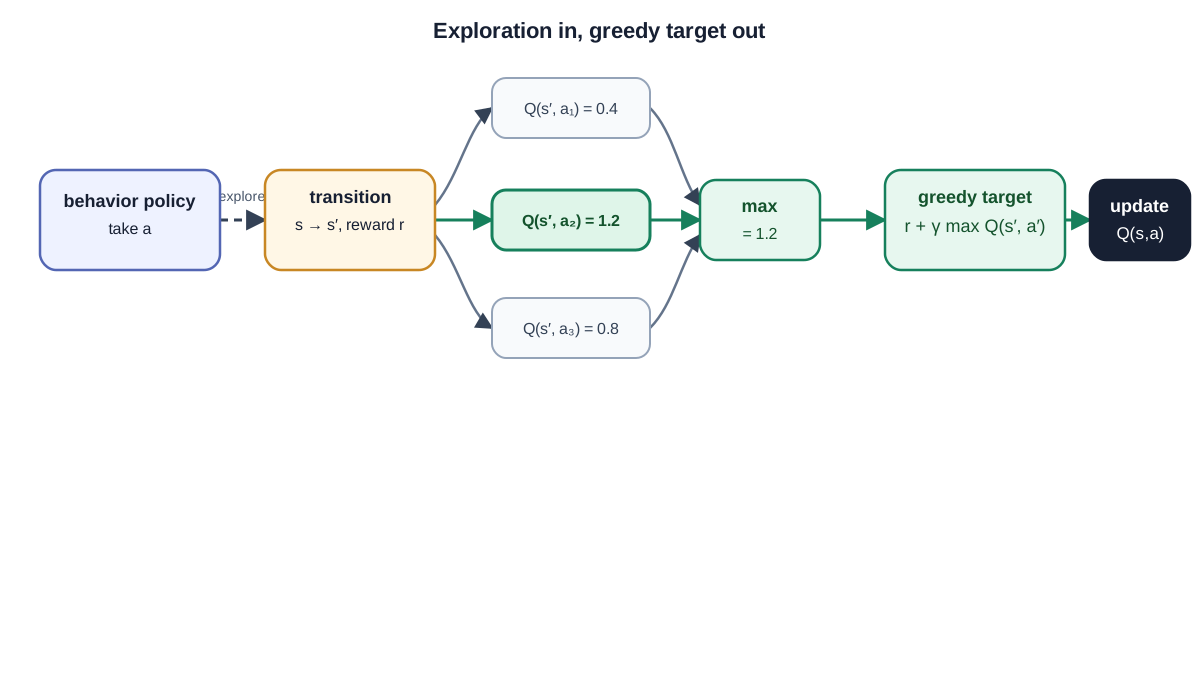
Here's the move that confuses everyone: the update never uses the action you actually took in the next state.
You took action a in state s. That action got you to s'. But when you build the target, you don't ask "what would my current behavior policy do next?" You ask "what is the best action available in s', according to my current table?"
That distinction separates two policies:
- Behavior policy: the policy that picks actions during data collection. It might be epsilon-greedy, mostly random, or even fully random.
- Target policy: the policy whose values you're learning. For Q-learning, that's the greedy policy—always take the action with the highest Q value.
The update learns the value of the greedy policy from data generated by whatever policy happened to explore. That's the off-policy property in one sentence.
Contrast this with SARSA, the on-policy cousin. SARSA's target uses the action the behavior policy actually selects in the next state:
Q(s, a) ← Q(s, a) + α [r + γ Q(s', a') − Q(s, a)]
where a' is chosen by the behavior policy. If your behavior policy is epsilon-greedy, SARSA learns the value of that epsilon-greedy policy, randomness included. Q-learning ignores what the behavior policy would do and substitutes the best action instead.
| Algorithm | Target uses | Learns the value of |
|---|---|---|
| Q-learning | max over next actions | Greedy policy |
| SARSA | action the behavior policy actually takes | Behavior policy (including its exploration) |
This is why Q-learning is off-policy: the data doesn't need to come from the policy being learned. A random policy generates transitions—state, action, reward, next state—and each transition carries information about the environment. Q-learning extracts that information and uses it to improve estimates of the greedy policy's value.
In practice, this property is what makes experience replay possible. You can store transitions in a buffer, sample them later in random order, and update from old data collected under older, more exploratory policies. Q-learning doesn't care where the transition came from.
Knowledge check
Check your understanding
Answer this question before you continue.
What Exploration Actually Buys You
The off-policy mechanism is powerful, but it has a hidden dependency: the max target is only as good as the estimates beneath it.
If a state-action pair is never visited, its Q value stays at whatever arbitrary value you initialized it to. If the max in your target points at an unvisited action with an inflated initial value, the target itself is garbage. The update faithfully moves your estimate toward a wrong number.
This is why exploration isn't a hack bolted onto Q-learning. It's a requirement for the max to mean anything.
Epsilon-greedy exploration exists for exactly this reason. With probability ε, the agent picks a random action instead of the greedy one. That randomness guarantees the agent eventually samples enough actions for the table to reflect reality rather than initialization values.
The practical failure mode is familiar: if ε decays too fast, the agent locks onto a locally good action early. The max target then keeps reinforcing a wrong belief because the better action never gets sampled enough to correct its estimate. The agent isn't learning that its choice is optimal. It's learning that its choice is the only one it ever tries.
One alternative worth knowing: optimistic initialization. Instead of relying on random exploration, initialize all Q values high. The first time the agent tries an action, the update pulls the estimate down toward reality. Actions that haven't been tried still look attractive, so the agent keeps sampling them. Exploration emerges from the update mechanism itself rather than from a separate random policy.
The cost of exploration is real. Every random action is a step where the agent isn't following its best current belief. That's the exploration-exploitation tradeoff showing up inside the algorithm. Q-learning's off-policy structure doesn't eliminate the tradeoff. It just makes the data from exploratory steps useful for learning the greedy policy instead of wasting it.
Knowledge check
Check your understanding
Answer this question before you continue.
Where Q-Learning Shines and Where It Stumbles
Q-learning is a workhorse for good reasons. It's model-free—no need to know the environment's transition dynamics. It handles discrete action spaces naturally. And its off-policy nature means you can reuse experience efficiently, which is what makes deep Q-learning with replay buffers feasible.
But it has honest weaknesses.
Overestimation bias. The max operator has a subtle flaw: it uses the same estimates to both select and evaluate the best action. In noisy environments, some actions will have inflated estimates by chance. The max picks the most inflated one, and the target inherits that inflation. Over many updates, Q values drift upward. The agent becomes overconfident about actions that look better than they are.
Double Q-learning fixes this by separating selection from evaluation: use one value function to pick the best action, and a second to estimate its value. The overestimation doesn't fully disappear, but it stops compounding.
The leap to function approximation. A table works when the state space is small enough to enumerate. Real problems—video frames, sensor readings, continuous control—have state spaces no table can hold. Replace the table with a neural network and you get DQN, a classic deep RL algorithm. But function approximation plus bootstrapping plus off-policy data creates instability. The same off-policy property that enables replay also makes training less stable, because the data distribution shifts as the policy improves. Taming that instability required target networks, replay buffers, and careful tuning.
When to Reach for Q-Learning (and When Not To)
Here's my practical decision rule:
Use Q-learning when you have discrete actions, no model of the environment, and you can tolerate learning from off-policy or replayed experience. If you have a simulator, a discrete action space, and a value surface a table or modest network can represent, Q-learning is a solid first choice.
Avoid it when you need a stochastic policy directly, when actions are continuous, or when you're learning from a fixed dataset that lacks coverage of the actions the max might rank highly. The max operator assumes you can eventually sample the actions it values. If your data is fixed and missing those actions, Q-learning will extrapolate badly from estimates that were never grounded in real experience.
Note the distinction: replay from a buffer you keep filling is fine, because new interaction can correct mistakes. A truly fixed dataset is different—if the good actions were rarely or never taken during collection, no amount of replay will manufacture the evidence the max needs.
For continuous actions or problems where you need a distribution over actions rather than a single best choice, policy-gradient and actor-critic methods are the natural next step. They optimize the policy directly instead of learning values and deriving a policy from them.
The Mental Model That Sticks
Here's the durable way to think about Q-learning: it learns the value of the best action from the data of whatever action was actually taken.
Every transition is evidence about the environment. Q-learning extracts that evidence, then asks a question that ignores how the evidence was collected: given where I landed, what's the best I could do next? The answer becomes the target, and the estimate moves toward it.
Try this yourself. Take a tiny grid—three states, two actions per state, one reward at the end. Initialize the table to zeros. Run a purely random policy for a few hundred steps, applying the Q-learning update after every transition. Then check two things: the Q values and how often each state-action pair was visited.
You'll notice the rewarding path's values climb only after the random policy stumbles into it enough times for the reward to propagate backward through the max. An action that was never tried will still sit at zero, invisible to the max because the agent never landed in a state where that action was available. The values that moved are the ones with evidence beneath them.
That's the off-policy magic, stated precisely: the agent never had to deliberately follow the right path to learn the value of the right path. It only had to visit the relevant states and actions often enough for the max to see the truth.
Knowledge check
Final check
Finish the article by checking the ideas you just learned.
References
Research updated Sep 9, 2026


