Monte Carlo vs Temporal-Difference Learning in Reinforcement Learning

Both methods learn from experience. One waits for the story to end before drawing conclusions. The other revises its belief after every sentence. The real difference is not timing—it is what each method trusts as the truth.

If you have worked through returns and discounting, you know that an agent's goal is to estimate how much reward it can expect from each state. The Bellman equation showed you that this value can be decomposed into an immediate reward plus a discounted continuation. Now comes the practical question: when the agent actually interacts with the environment, how should it turn those interactions into better estimates?

Monte Carlo and temporal-difference learning answer that question differently. Understanding the difference is not about memorizing two update rules. It is about choosing what to trust.

The Question Behind the Comparison

Imagine you are teaching someone to estimate how long their commute will take. One approach: wait until they arrive, look at the total time, and adjust their estimate based on the full trip. Another approach: after the first five minutes, look at how far they have gotten, make a prediction about the rest of the trip, and adjust immediately.

Both approaches use real experience. Neither one requires a map of the city. But they trust different evidence.

Monte Carlo (MC) methods trust the measured return—the actual sum of discounted rewards collected over an entire episode. Temporal-difference (TD) methods trust something thinner: the reward observed in the next step, plus a discounted guess about the value of the state that follows.

That single difference cascades into everything else: when updates happen, how noisy they are, whether they can learn from incomplete episodes, and whether the final estimates carry bias.

Monte Carlo: Waiting for the Full Return

Monte Carlo reinforcement learning is the patient method. The agent plays through an entire episode—from start to finish—and only then looks back at what happened.

Suppose a gridworld agent starts in the top-left corner, wanders through a few rooms, collects a reward, and finally reaches the goal. At the end, the agent sums up all the discounted rewards it collected after each state. That sum, called the return ( G_t ), becomes the update target for every state visited along the way.

The appeal is straightforward: the return is a real measurement. It is not a guess. It is what actually happened when the agent followed its policy. Because it is a genuine sample of the true value, the MC target is unbiased. If you ran the same policy many times and averaged the returns, you would converge to the correct value.

But that measurement comes at a cost. The return depends on a long chain of random events: every transition, every reward, every lucky or unlucky turn. One episode might end with a huge reward because the agent stumbled into a favorable sequence. The next episode might end badly through no fault of the policy. The variance is high, and averaging out that noise requires many episodes.

There is also a structural limitation. Standard episodic Monte Carlo cannot make its usual complete-return update until a stopping point exists. If your task is a game that always ends, that is fine. If your task is a continuing process—a robot arm that runs all day, a trading agent that never sees a natural stopping point—there is no finish line to wait for. The practical issue is not that MC has no relationship to continuing experience; it is that the method's update target depends on a return that never arrives.

Temporal-Difference: Updating From a One-Step Guess

Temporal-difference learning takes the other path. After a single transition—one state, one action, one reward, one next state—the agent already has enough to update.

The TD target is the observed reward ( R_{t+1} ) plus the discounted current estimate of the next state's value: ( R_{t+1} + \gamma V(S_{t+1}) ). The agent takes one real step into the future, then leans on its own estimate for everything beyond that.

This is bootstrapping. The update uses an existing estimate as part of its own target. The agent is not waiting for the ground truth; it is revising its belief based on a small piece of reality plus a guess.

That guess is the source of both TD's strength and its weakness.

Because the TD target depends on only one reward and one transition, it carries far less variance than a full return. The learning signal is smoother, less sensitive to individual noisy episodes, and often converges faster in practice. TD also learns online—after every step—which makes it the natural choice for continuing tasks that never end.

The cost is bias. Early in learning, the estimate ( V(S_{t+1}) ) is likely wrong. The agent is updating toward a target that contains an error. If those bootstrapped estimates stay wrong—especially when combined with function approximation—TD can converge to the wrong answer.

Watching the Update Move

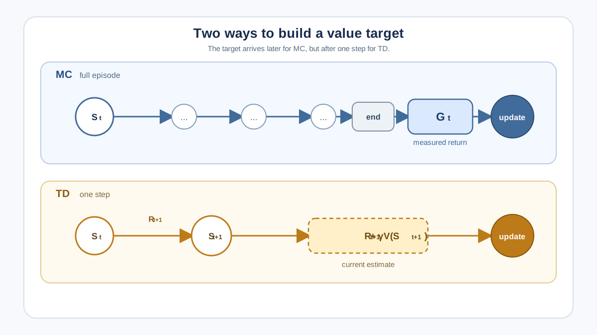
The distinction becomes concrete when you watch the numbers change. Suppose the agent is in state ( S_t ), and its current estimate is ( V(S_t) = 5 ). It takes one step, receives reward ( R_{t+1} = 0 ), and lands in a state the agent currently values at ( V(S_{t+1}) = 8 ). With a discount factor of ( \gamma = 0.9 ), the TD target is:

[ R_{t+1} + \gamma V(S_{t+1}) = 0 + 0.9 \times 8 = 7.2 ]

The TD error is the gap between this target and the current estimate:

[ 7.2 - 5 = 2.2 ]

With a learning rate of ( \alpha = 0.1 ), the new estimate becomes:

[ V(S_t) \leftarrow 5 + 0.1 \times 2.2 = 5.22 ]

Notice what happened. The agent did not wait to discover whether the episode ends well or badly. It moved its estimate from 5 toward 7.2 based on one observed reward and a guess about the next state. The update is deliberately partial—it takes a small step toward a provisional target, not a leap to a final answer.

Contrast that with Monte Carlo. If the same episode continued for several more steps and ended with a measured return of ( G_t = 9 ), the MC update would move the estimate from 5 toward 9 in one step:

[ V(S_t) \leftarrow 5 + 0.1 \times (9 - 5) = 5.4 ]

TD is not claiming that 7.2 is the true return. It is claiming that 7.2 is a reasonable one-step target worth moving toward, given what the agent currently believes. That is why TD can update before the episode ends—and why its target carries bias until those beliefs improve.

First compute the target 0 + 0.9 × 8, then move the current estimate a fraction α toward that target.

Bias, Variance, and the Learning-Rate Tradeoff

The statistical contrast between Monte Carlo and temporal-difference learning is the cleanest way to hold the two methods in your head.

	Monte Carlo	Temporal-Difference (TD)
Update target	Complete return ( G_t )	One-step reward plus discounted estimate: ( R_{t+1} + \gamma V(S_{t+1}) )
When updates happen	After episode ends	After every step
Bias	Unbiased	Biased (leans on possibly wrong estimates)
Variance	High (long chain of random events)	Lower (fewer random events per update)
Data requirement	Needs complete episodes	Works with single transitions
Continuing tasks	No complete return to use as a target	Learns naturally

To make bias and variance operational, think about repeated runs. Monte Carlo targets are built from many random events, so individual targets scatter widely around the true value. Average enough of them and the noise cancels out—that is low bias with high variance. TD targets depend on fewer random events, so they scatter less. But they are pulled toward whatever the current estimate believes, which can be systematically wrong early in learning—that is lower variance with bias.

The learning rate interacts with this tradeoff. Because MC's target is unbiased, each update points in the right direction on average, so larger steps do not accumulate a systematic error. TD's target contains bias, especially early on, so smaller steps give the estimates time to improve before the agent commits too strongly to provisional guesses.

If you are debugging a learning curve that looks like static, you are probably watching high variance—the Monte Carlo pattern. If the curve looks smooth but settles at the wrong level, bias may be the culprit—a pattern TD can show when bootstrapped estimates stay wrong. These are diagnostic possibilities, not guaranteed signatures. Plot shape alone rarely tells the full story.

When Each Method Earns Its Keep

My rule of thumb: reach for Monte Carlo when you need an unbiased measurement of a fixed policy, and reach for temporal-difference when you need to learn online.

Monte Carlo earns its keep in policy evaluation. If you have trained an agent and want to compare it against another agent, you want an unbiased measurement of true performance. Run each policy to completion, average the returns, and you have a trustworthy comparison. This is also why Monte Carlo is a good first implementation for learning: it is conceptually simple, easy to debug, and the target is transparent. You can see exactly what the agent is updating toward.

One condition matters here: this evaluation advice assumes you can run complete episodes under the policy being measured. If the policy keeps changing during data collection, or if episodes never end, the measurement setup needs more care.

Temporal-difference earns its keep when you need incremental learning. When episodes are long, waiting for completion wastes experience. When rewards are noisy, TD's lower variance smooths the learning signal. When the task is continuing, TD is the practical choice of the two because its update does not depend on a final return. And in value-based control, TD is the engine behind Q-learning and SARSA—the methods that learn optimal policies from single transitions.

There is an honest boundary worth stating. TD's bias becomes a genuine problem when you combine bootstrapping with function approximation. The interaction between the two can cause instability or divergence. That is a later topic, but it is why the choice between MC and TD is not settled once and for all—it depends on what you are building.

Common Misconceptions to Drop

"TD is always better than MC." No. TD's bias can lead it astray, and Monte Carlo's unbiased target is genuinely valuable for evaluation. The two methods have different statistical profiles, not different ranks.

"Bootstrapping means TD ignores real rewards." It does not. The TD target includes the observed reward ( R_{t+1} ). It combines that real measurement with a guess about the future. TD ignores nothing; it just refuses to wait.

"The difference is only about speed." Speed is a symptom. The deeper difference is what each method trusts as its target—a measured return versus a bootstrapped estimate—and that choice drives the entire bias-variance profile.

"MC and TD are mutually exclusive." They are endpoints on a spectrum. TD(λ) blends them by controlling how far credit travels across time. At one extreme, it behaves like Monte Carlo; at the other, like one-step TD. The comparison you are learning now is the foundation for that later idea.

The Decision Rule

When you need an unbiased measurement of a fixed policy and complete episodes are available, reach for Monte Carlo. When you need to learn online from noisy or continuing experience, reach for temporal-difference.

The next natural step is seeing how bootstrapping powers Q-learning—how the TD target extends from state values to action values, and how that shift enables agents to learn optimal policies without a model of the environment. That is where the comparison you just built starts doing real work.

References

Research updated Sep 9, 2026