
Derive Cumulative Regret in a Finite Contextual Bandit
A policy that earns more reward is not automatically a better policy. It may just have met easier contexts.

Key topics
A policy that earns more reward is not automatically a better policy. It may just have met easier contexts.
You run an epsilon-greedy contextual bandit. Total reward climbs. You conclude the algorithm is working. Then you change the context distribution, rerun the same code, and the total reward drops by half. Nothing about the algorithm changed. The contexts changed.
That is the trap. Total reward is a number without a denominator. It depends on how easy the contexts happened to be, how noisy the rewards were, and how long you ran. It cannot tell you whether your policy is learning anything.
Regret changes the question. Instead of asking "how much did I earn?", it asks "how much did I leave on the table compared to a stated benchmark?" That benchmark is called the comparator, and every regret number is meaningless until you name it.
One qualification before we go further, because it is easy to overclaim here. Regret controls for context difficulty when the policy and the oracle are scored on the same encountered contexts. It does not normalize away the context mix. Two regret values computed on different context sequences are still answering different questions. Keep that in mind every time you compare numbers across runs.
By the end of this article, you will define per-round regret against a context-aware oracle, derive cumulative regret as a sum of gaps, and compute it by hand for a tiny finite problem. You will also see exactly which assumptions make that number mean something.
This assumes you already know the contextual-bandit loop: context arrives, you pick one action, you observe one reward, no state transition. If that loop is fuzzy, the bandit-versus-RL comparison is the right place to start. Here we take the loop as given and focus on measuring it.
Why Total Reward Is the Wrong Scoreboard
Two policies can earn identical total reward on different context sequences and still differ wildly in quality. A lucky sequence of easy contexts inflates reward without any learning having occurred. An unlucky sequence punishes a good policy.
The fix is not a better reward metric. It is a comparison. Measure the gap between what you earned and what a fixed reference would have earned on the same contexts.
That reference is the diagnostic handle for this entire article. I call it the comparator. Change the comparator, and you change the number. Compare two regret values from different papers or implementations without checking that the comparators match, and you are comparing apples to a different orchard.
Notation: Contexts, Actions, and Expected Rewards
Before any derivation, define every symbol. Keep this tight — you already know the setting, you just need shared vocabulary.
At each time step :
- A context arrives from a finite context set .
- The agent picks an action from a finite action set .
- The environment returns a reward , a noisy draw around an expected value.
The expected reward for taking action under context is . The observed reward is a random draw whose mean is .
Two derived quantities matter:
- The best action for a context: .
- The best achievable mean reward for that context: .
Why work with expected rewards instead of realized draws? Because regret is defined on means. Noise averages out, and the gap reflects policy quality rather than luck. If you define regret on a single noisy trajectory, one outlier reward can dominate the entire sum.
Flag the finite assumption now: finite context set, finite action set, bounded rewards. Each of these returns in the assumptions section, because each one is load-bearing.
Knowledge check
Check your understanding
Answer this question before you continue.
The Oracle Comparator: What "Optimal" Actually Means
The comparator here is the context-aware oracle. It knows for every pair and always plays .
The oracle is a benchmark, not an achievable algorithm. It already knows the answer. No real agent can match it, because a real agent has to learn from noisy observations. That is the point: the oracle gives you a fixed ceiling to measure against.
Per-round regret is the gap at a single step:
It is zero when you happen to pick the best action, and positive otherwise. Simple, but the choice of comparator is a modeling decision, not a formality.
Some bandit work uses a weaker comparator: the best fixed policy in a restricted policy class. Regret against a fixed-policy benchmark is a different, generally smaller number than regret against the per-context oracle. Both are legitimate. They answer different questions. If your policy class cannot express the per-context optimum, measuring against the oracle will show a gap your algorithm can never close.
Common mistake: Reading a regret number without checking which comparator produced it. A small regret against a weak comparator is not evidence of a strong policy.
One more distinction worth naming: simple regret versus cumulative regret. Simple regret is the final gap — how far from optimal you are at the end. Cumulative regret is the sum of gaps along the way. Minimizing one is not the same objective as minimizing the other. An algorithm tuned for a small final gap is not automatically good at keeping the running sum small. This article is about the cumulative version.
Knowledge check
Check your understanding
Answer this question before you continue.
Cumulative Regret as a Sum of Gaps
Now derive the quantity. Start from the per-round gap:
Cumulative regret is the sum over the horizon:
That is the whole derivation. Two lines. The work is in interpreting it.
is the total expected reward you left on the table by not playing the oracle's action every round. It is a cost, not a score. Lower is better. And it is a sum rather than an average because the sum is what accumulates against you over a horizon — it is the quantity that regret bounds are stated for.
For any suboptimal action, define the gap:
Your per-round regret is exactly the gap of whatever action you chose. So is a sum of gaps you incurred, one per round.
A Hand-Computed Example
Three contexts, two actions. Here is the expected reward table:
| Context | ||||
|---|---|---|---|---|
| 1.0 | 0.4 | 1.0 | ||
| 0.3 | 0.9 | 0.9 | ||
| 0.6 | 0.6 | 0.6 | either |
The context sequence over rounds is:
Suppose your policy plays this action sequence:
Compute the per-round gap for each step:
| 1 | 1.0 | 1.0 | 0.0 | ||
| 2 | 0.3 | 0.9 | 0.6 | ||
| 3 | 1.0 | 1.0 | 0.0 | ||
| 4 | 0.6 | 0.6 | 0.0 | ||
| 5 | 0.9 | 0.9 | 0.0 | ||
| 6 | 1.0 | 1.0 | 0.0 |
Sum the gaps:
The entire regret comes from round 2, where the policy played under context and left 0.6 of expected reward behind. Every other round was optimal.
This is the anchor example. Keep it in view for the next section.
Knowledge check
Check your understanding
Answer this question before you continue.
Worked Example: Greedy Versus Exploring on the Same Sequence
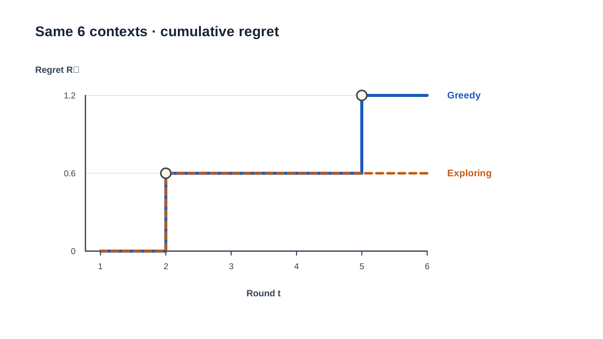
Now replay the identical context sequence under two policies. Same contexts, same reward table, different decisions.
Greedy policy. It estimates from the first observation it gets for each context-action pair and then commits. Suppose its first observation under happens to be a noisy draw from that looks good. It locks onto for and never revisits.
Epsilon-greedy policy. It mostly exploits but occasionally probes with probability . The probe under eventually reveals that is better.
Here is a plausible action sequence for each over the same six rounds:
| Greedy | Greedy | Exploring | Exploring | ||
|---|---|---|---|---|---|
| 1 | 0.0 | 0.0 | |||
| 2 | 0.6 | 0.6 | |||
| 3 | 0.0 | 0.0 | |||
| 4 | 0.0 | 0.0 | |||
| 5 | 0.6 | 0.0 | |||
| 6 | 0.0 | 0.0 |
Greedy cumulative regret: .
Exploring cumulative regret: .
Read this table carefully, because it is easy to over-interpret. These are stipulated action sequences, not a simulation of a learning algorithm. I chose them to isolate one variable: what happens to when a policy keeps repeating a mistake versus when it corrects one. The table shows the arithmetic of regret, not proof that exploration discovered anything.
To see the mechanism that would actually produce the exploring sequence, trace the smallest possible feedback loop. Suppose the agent's estimate for starts at 0.3 and its estimate for starts at 0.5 — a rough prior. At round 2 it plays and observes a reward near 0.3, so the estimate for stays low. At round 4, an -probe fires under and the agent plays ; the reward near 0.6 nudges the estimate upward. By round 5, the estimate is now the higher one for , so the greedy step inside epsilon-greedy selects . That single observation is what flips the decision. The exploring policy did not get lucky; it paid for information and then spent it.
Now look at the mechanism in the regret column. Both policies paid the same 0.6 gap at round 2. The greedy policy kept paying it every time reappeared, because it never corrected its estimate. Its per-round gap persisted, so its grew linearly with the number of visits. The exploring policy paid the same early gap, then drove its per-round gap to zero once the estimate flipped. Its stopped growing.
That is the whole story of exploration in one table. Exploration is an investment in reducing future gaps. Regret is the accounting that tells you whether the investment paid off. If you plot cumulative regret over for both policies, greedy is a line with a persistent positive slope; exploring is a line that flattens after the probe. The slope change is where the estimate changed.
Knowledge check
Check your understanding
Answer this question before you continue.
Assumptions That Make Mean Something
A number is not a guarantee. Here is what has to hold before you can interpret as one.
Bounded rewards. If rewards are unbounded, a single outlier draw can dominate the sum. stops being a stable performance measure and starts being a story about one lucky or unlucky round.
Stationarity. The table assumes is fixed. If the environment drifts — user preferences change, a recommendation model's audience shifts — past experience misleads the agent, and the oracle benchmark itself moves. Regret against a moving target is a different problem.
Correct comparator. is only interpretable relative to the oracle you declared. A smaller against a weak comparator is not evidence of a better policy.
Finite sets. Finite contexts and actions keep the example computable by hand. Infinite or continuous action spaces change both the algorithm design and the shape of the achievable bounds.
Matched context distribution. Regret is measured on the contexts that actually arrive. Change the context mix, and you change the question, even if the algorithm and the reward table are identical. Comparing across runs with different context distributions is only meaningful if you say so explicitly.
What a regret bound does and does not promise. A sublinear regret bound says the expected cumulative gap grows slower than the horizon under stated conditions. It is not a per-run guarantee. It says nothing about any single observed trajectory. It does not promise the agent will be near-optimal soon — that depends on the constant, the horizon, and the gap structure.
Common mistake: Reading "sublinear regret" as "the agent will be near-optimal soon" without checking the constant, the horizon, and how large the gaps actually are. A bound with a huge constant can be technically sublinear and practically useless at your scale.
From to a Practical Reading Habit
Before you trust any regret number, ask three questions:
- What comparator? Oracle, best fixed policy, or something else?
- What horizon? at and are different claims.
- What reward bounds? Bounded rewards make the sum stable. Unbounded rewards make it fragile.
When you log an experiment, log the per-round gap alongside the reward. The reward tells you what you earned. The gap tells you whether learning is happening. Those are different signals, and only one of them survives a change in context difficulty.
Regret is the right lens for bandit-style problems because actions do not change future states. Once actions shape the state the agent sees next, the per-step oracle stops capturing the problem — you cannot evaluate a decision in isolation when it changes what comes after. That transition is the move from bandits into full reinforcement learning, and it is where temporal-difference methods and credit assignment take over.
Here is your next move. Take the three-context table above. Change from 0.3 to 0.1, so the greedy policy's mistake becomes more costly. Recompute for both policies. Watch how the gap structure — not the algorithm label — drives the result. Then change the context sequence so appears only once. The greedy policy's regret collapses. Same algorithm, same mistake, different cost, because the context distribution changed.
That is the lesson worth keeping: regret measures a policy against a declared benchmark on a declared context distribution. Change either, and you have changed the question.
Knowledge check
Final check
Finish the article by checking the ideas you just learned.
References
Build a stronger RL mental model
Use structured resources to connect equations, algorithms, and observable agent behavior.


