Deriving Discounted Return: How Future Rewards Become an Objective

You already know the feeling: a reward now beats the same reward later. This article turns that feeling into a formula you can defend, compute, and eventually optimize.

From a Reward Sequence to a Single Number

Here is the setup. An agent acts, the environment responds, and a reward arrives. Then it happens again. And again. What you get is a sequence:

$r_0, r_1, r_2, r_3, \dots$

Each $r_t$ is the reward received at time step $t$. That sequence is the raw material. But a sequence is not an objective. You cannot rank two policies by comparing two lists of numbers of different lengths, with different timings, and different totals. To choose between policies, you need one number per trajectory — a scalar you can compare, average, and maximize.

That number is the return, written $G_t$. The return is the cumulative reward the agent collects starting from time step $t$. If you have read the intuition-level treatment of rewards and discounting, you already know the shape of this idea. What we are doing here is different: we are going to build the formula term by term, so that every power of $\gamma$ appears for a reason instead of arriving as a memorized pattern.

Before we write anything down, let me fix the notation, because sloppy notation is where most of the confusion starts:

• $t$ — the time index. A counter that ticks forward one step at a time.
• $r_t$ — the reward received at step $t$.
• $\gamma$ — the discount factor, a constant in the interval $[0, 1)$. It is fixed for the whole task, not something the agent learns.
• $G_t$ — the return from step $t$ onward.

That last symbol is the one we are deriving. Everything else is scaffolding.

Why Undiscounted Sums Break Down

The naive objective is the plain sum: add up every reward the agent ever receives. It sounds right. It fails for two separate reasons, and it is worth keeping them apart.

The first reason is convergence. In a continuing task — one that never ends — the sum runs forever. If the agent keeps collecting any positive reward, the total keeps growing without bound. There is no finite number to maximize. You cannot optimize a quantity that never settles.

The second reason is preference. Even when the sum is finite, a plain sum treats a reward a thousand steps away as exactly as valuable as a reward right now. For most tasks, that is the wrong priority. If you are steering a car, a crash in ten seconds matters more than a crash in ten minutes, and not only because the episode might end first.

Discounting fixes both problems with one mechanism. Each reward is multiplied by a weight that shrinks as the reward moves further into the future. The weight on a reward $t$ steps away is $\gamma^t$. Because $\gamma$ is less than one, those weights get smaller and smaller, which both keeps the infinite sum finite and encodes the preference for earlier reward.

Note: Discounting is a modeling choice, not a law of nature. You are deciding how much the future should count. That decision has consequences, and we will come back to them.

Deriving the Discounted Return Step by Step

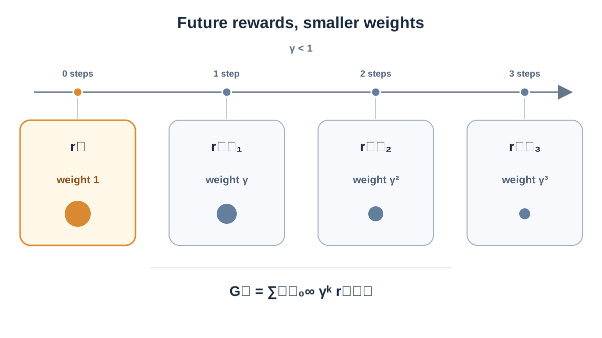
Let us build the formula from the first term outward.

Start at time step $t$. The reward you receive right now is $r_t$. How much weight should it carry? None of it is in the future, so it is not discounted at all. Its weight is $\gamma^0 = 1$.

$G_t = r_t + \dots$

One step later, the reward is $r_{t+1}$. It is one step into the future, so it gets one factor of $\gamma$.

$G_t = r_t + \gamma r_{t+1} + \dots$

Two steps later, the reward is $r_{t+2}$, two steps into the future, so it gets two factors of $\gamma$.

$G_t = r_t + \gamma r_{t+1} + \gamma^2 r_{t+2} + \dots$

The pattern is now visible. A reward received $k$ steps after $t$ carries weight $\gamma^k$. Writing the full sum:

$G_t = r_t + \gamma r_{t+1} + \gamma^2 r_{t+2} + \gamma^3 r_{t+3} + \dots = \sum_{k=0}^{\infty} \gamma^k r_{t+k}$

Read that sum slowly. The index $k$ is the time offset from the present, not the absolute time. The exponent on $\gamma$ is always the offset. That is the whole trick: the further a reward sits from now, the more times you multiply it by a number smaller than one.

The Recursive Form

There is a second way to write the same thing, and it matters more than it looks. Pull the first term out of the sum:

$G_t = r_t + \gamma \left( r_{t+1} + \gamma r_{t+2} + \gamma^2 r_{t+3} + \dots \right)$

The part in parentheses is exactly $G_{t+1}$ — the return starting one step later. So:

$G_t = r_t + \gamma G_{t+1}$

This is the recursive form of the return. The return from here equals the reward I get now, plus the discounted return from wherever I land next. That self-reference is not a curiosity. It is the seed of every Bellman-style equation you will meet later, because it lets you express the value of a state in terms of the values of the states that follow it.

Why the Infinite Sum Converges

The sum $\sum_{k=0}^{\infty} \gamma^k r_{t+k}$ is only useful if it lands on a finite number. Two conditions get us there.

First, rewards must be bounded. There is some maximum absolute reward $R_{\max}$ that the environment can hand out. This is true in essentially every practical task — rewards are numbers produced by a reward function, and reward functions do not return infinity.

Second, $\gamma < 1$. With both conditions, the sum is squeezed by a geometric series:

$|G_t| \le \sum_{k=0}^{\infty} \gamma^k R_{\max} = \frac{R_{\max}}{1 - \gamma}$

That right-hand side is finite whenever $\gamma < 1$. The return cannot run away, no matter how long the task continues.

Warning: If $\gamma = 1$ in a continuing task, the bound becomes $R_{\max} / 0$ — meaningless. There is no convergence guarantee, and the objective may not exist. Setting $\gamma = 1$ is only safe when the task provably ends.

From One Trajectory to the Objective a Policy Maximizes

So far we have a number for a single trajectory. But the agent does not get to pick one trajectory and keep it. It picks a policy, and the policy generates trajectories. Different runs produce different reward sequences, because transitions and sometimes actions are random.

That is why the objective is not $G_0$ itself. The objective is the expected return — the average of $G_0$ over all the trajectories the policy could produce:

$\max_{\pi} \; \mathbb{E}_{\pi}\left[ G_0 \right]$

Read the pieces. $\pi$ is the policy, the agent's rule for choosing actions. The expectation $\mathbb{E}_{\pi}$ averages over the randomness in the environment and in the policy's own choices. $G_0$ is the discounted return from the start. The agent is not trying to make one lucky run look good; it is trying to make the average run good.

This distinction matters the moment you start reading algorithms. A single $G_t$ is a sample. The expected return is the thing being optimized. Value functions are the bridge between them: $V(s)$ and $Q(s, a)$ estimate the expected return you would collect starting from a state or a state-action pair, which is exactly the quantity the policy is trying to push upward.

Common mistake: Confusing a high return on one episode with a good policy. A policy is judged by its expected return across many episodes, not by its best single run.

Worked Example: Discounting a Short Reward Sequence

Numbers make this concrete. Suppose the agent receives rewards $r_0 = 1$, $r_1 = 2$, $r_2 = 3$, and then the episode ends. Take $\gamma = 0.9$.

Write each term with its weight:

$G_0 = \gamma^0 (1) + \gamma^1 (2) + \gamma^2 (3)$

Compute the weights: $\gamma^0 = 1$, $\gamma^1 = 0.9$, $\gamma^2 = 0.81$. Now the arithmetic:

$G_0 = 1 + 0.9(2) + 0.81(3) = 1 + 1.8 + 2.43 = 5.23$

Now the same rewards with $\gamma = 0.5$. The weights become $1$, $0.5$, and $0.25$:

$G_0 = 1 + 0.5(2) + 0.25(3) = 1 + 1.0 + 0.75 = 2.75$

Same rewards. Same order. Different objective. The lower discount factor shrinks the later contributions hard: the third reward drops from $2.43$ to $0.75$, while the first reward is untouched in both cases.

$\gamma$	Weight on $r_0$	Weight on $r_1$	Weight on $r_2$	Return
0.9	1.00	0.90	0.81	5.23
0.5	1.00	0.50	0.25	2.75

A sanity check you can run on any return: it always sits between the undiscounted sum and the first reward alone. Here the undiscounted sum is $6$, and the first reward is $1$. Both $5.23$ and $2.75$ fall inside that range, as they must.

How Task Structure Changes the Objective

The formula is the same. What it means depends on whether the task ends.

In an episodic task, the interaction runs until a terminal state, then resets. The horizon is finite, so the sum has a natural stopping point. Because the sum is finite, $\gamma = 1$ is mathematically available — the undiscounted return will not diverge. But available is not the same as appropriate. Discounting still encodes a preference for earlier reward, and whether you want that preference depends on the task, not on whether episodes happen to end. If every reward through termination should count equally, $\gamma = 1$ matches your intent. If a reward ten steps before the end should matter less than one now, keep $\gamma < 1$ even though the episode is finite.

In a continuing task, there is no terminal state. The agent runs forever. Here discounting is what keeps the objective well-defined. An alternative is an average-reward formulation, which measures reward per step rather than a total, but the discounted return is the standard practical objective and the one most value methods assume.

Task type	Horizon	Is $\gamma < 1$ required?	What the return represents
Episodic	Finite, ends at terminal state	No, but still a modeling choice	Total reward until the episode ends
Continuing, discounted	Infinite	Yes	Weighted total, with future rewards shrunk
Continuing, average-reward	Infinite	Not applicable	Reward per step, in the long run

The decision rule I use: first ask what the task actually values. If all rewards through termination should count equally, an undiscounted episodic return is defensible. If earlier rewards should matter more, discount — even in an episodic task. If the task runs forever, discounting is the default, because without it you have no finite number to maximize.

One practical blur worth knowing about. Algorithms frequently optimize one formulation while estimating values with another — for example, optimizing the undiscounted return but using a discount factor inside the value function. This is common enough that you should read the objective in the code, not assume it from the paper's framing.

What the Derivation Buys You

The return is not an abstraction that lives only in this article. It is the quantity that value functions estimate. $V(s)$ and $Q(s, a)$ are expectations of $G_t$ — the average return you would collect starting from a state or a state-action pair. Every value method you meet next is, at bottom, trying to predict the number we just derived.

Discounting also shapes behavior in ways you can see. A low $\gamma$ produces a myopic agent that grabs nearby reward and ignores distant consequences. A high $\gamma$ produces a far-sighted agent that will accept short-term pain for long-term gain. Change $\gamma$, and the policy changes with it.

Common mistake: Treating $\gamma$ as a hyperparameter to tune until the numbers look good. It is a statement about how much the future should count. Tune it, yes — but know what you are claiming when you do.

Common mistake: Assuming a larger $\gamma$ always means a better agent. A high discount factor can also mean slower, noisier learning, because the agent is now responsible for a longer and less certain chain of consequences.

Where This Leads Next

Before you write or read any RL objective, do two things. First, identify whether the task is episodic or continuing. Second, choose $\gamma$ deliberately, because that choice defines what the agent is actually optimizing. Everything downstream inherits it.

The recursive form $G_t = r_t + \gamma G_{t+1}$ is your next tool. It is the step that turns a definition of return into Bellman-style value targets, where the value of a state is written in terms of the values of the states that follow.

Here is a small exercise that will teach you more than rereading this article. Recompute the worked example with $\gamma = 0.99$ and again with $\gamma = 0.1$. Before you run the arithmetic, predict which reward dominates in each case, and what kind of policy each discount factor would produce. Then check your prediction against the numbers. When your prediction and the arithmetic agree, you own the concept.