Compare Discounted and Average Reward in a Continuing RL Task

You tune gamma, the policy looks fine on your dashboard, and the task never ends. That is exactly when the scoreboard you optimized and the scoreboard you care about can disagree.

This is a small, runnable experiment. We will build a continuing process with no terminal state, define two fixed policies, and score each one under two objectives: the discounted return and the long-run average reward. Then we will watch the rankings move as gamma changes.

You should already know what a return is, what discounting does, and what a value function predicts. If those are shaky, the earlier material on rewards, returns, and discounting covers the ground we are standing on. Here we only need the two definitions side by side.

A discounted return sums rewards with a weight that shrinks with distance: r_0 + gamma*r_1 + gamma^2*r_2 + .... The average-reward objective asks a different question: in the limit, how much reward do I collect per step? In a continuing task, the discounted sum can be finite and well-behaved while the average reward is the number an operator would actually measure off the machine.

This is a tabular experiment with known dynamics. No function approximation, no learning algorithm, no neural network. We are evaluating fixed policies, which keeps the disagreement between objectives visible instead of tangled up with optimization noise.

Design a Continuing Process With No Terminal State

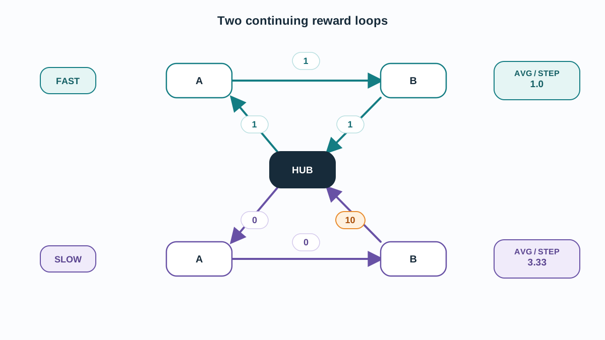
We need an environment small enough to reason about by hand and rich enough to expose a disagreement. The shape that does this is a fast loop that pays a little every step and a slow loop that pays more but rarely.

Here is the process. Five states, two actions, no absorbing state. Every step continues.

import numpy as np

# States: 0 = hub, 1 = fast loop A, 2 = fast loop B,
#         3 = slow loop A, 4 = slow loop B
# Actions: 0 = "fast" branch, 1 = "slow" branch

# Deterministic transitions: transitions[state][action] -> next_state
transitions = {
    0: {0: 1, 1: 3},
    1: {0: 2, 1: 2},
    2: {0: 0, 1: 0},
    3: {0: 4, 1: 4},
    4: {0: 0, 1: 0},
}

# Reward collected on entering the next state
rewards = {
    (0, 0): 1.0,   # hub -> fast loop A
    (0, 1): 0.0,   # hub -> slow loop A
    (1, 0): 1.0,   # fast loop A -> B
    (1, 1): 1.0,
    (2, 0): 1.0,   # fast loop B -> hub
    (2, 1): 1.0,
    (3, 0): 0.0,   # slow loop A -> B
    (3, 1): 0.0,
    (4, 0): 10.0,  # slow loop B -> hub
    (4, 1): 10.0,
}

Read the structure. The fast loop is hub -> 1 -> 2 -> hub: three steps, and it pays 1.0 on each step. That is 3.0 reward per 3 steps, or 1.0 per step.

The slow loop is hub -> 3 -> 4 -> hub: three steps, and it pays 0.0, 0.0, then 10.0. That is 10.0 reward per 3 steps, or about 3.33 per step.

So the slow loop has the higher per-step rate. But the fast loop pays immediately, and the slow loop makes you wait two steps before the payoff lands. That is the whole tension. A policy that reaches reward quickly can beat a policy with a higher steady-state rate when gamma is small.

The process runs for a fixed horizon T for estimation purposes only. The environment itself has no end.

Write the Two Estimators

The smallest useful code takes a policy, runs a rollout, and returns the reward sequence. Everything else is arithmetic on that sequence.

def rollout(policy, start_state=0, T=2000):
    """Run T steps. policy is a dict: state -> action."""
    state = start_state
    reward_seq = []
    for _ in range(T):
        action = policy[state]
        r = rewards[(state, action)]
        reward_seq.append(r)
        state = transitions[state][action]
    return reward_seq

def discounted_return(reward_seq, gamma):
    """Sum of gamma^t * r_t."""
    total = 0.0
    weight = 1.0
    for r in reward_seq:
        total += weight * r
        weight *= gamma
    return total

def average_reward(reward_seq):
    """Mean reward per step over the horizon."""
    return float(np.mean(reward_seq))

Two implementation choices matter here.

First, the average is taken over the full horizon, not a tail window. That is deliberate. It keeps the estimator honest about the transient from the start state, which we will use as a debugging signal later. If you take a tail window, you hide the bias instead of seeing it.

Second, the discounted sum is sensitive to gamma and the average is not. Gamma changes the weighting; the mean does not care about ordering at all. That asymmetry is the source of everything that follows.

Both numbers are estimates, not exact values. The discounted sum is exact for a deterministic process and a fixed horizon, but the average reward is a limit quantity that we are approximating with a finite mean.

Note: The average-reward estimate carries a transient bias from the start state. The horizon must be long enough for that bias to wash out. If your ranking changes when you extend T, the horizon is too short.

Run the Comparison and Read the Ranking

Define two fixed policies by hand. This keeps the comparison about objectives, not about learning.

policy_fast = {0: 0, 1: 0, 2: 0, 3: 0, 4: 0}
policy_slow = {0: 1, 1: 1, 2: 1, 3: 1, 4: 1}

policy_fast always takes the fast branch. policy_slow always takes the slow branch. Each policy commits to one loop and never leaves it.

Now score them.

policies = {"fast": policy_fast, "slow": policy_slow}
gamma = 0.5
T = 2000

for name, pol in policies.items():
    seq = rollout(pol, T=T)
    dr = discounted_return(seq, gamma)
    ar = average_reward(seq)
    print(f"{name:6s} discounted={dr:8.2f}  average={ar:6.3f}")

Expected output:

fast   discounted=    2.00  average= 1.000
slow   discounted=    2.86  average= 3.333

Read that carefully. At gamma = 0.5, the slow policy wins both comparisons. It wins the average-reward comparison by more than three to one: 3.333 against 1.000. It also edges out the fast policy on discounted return: 2.86 against 2.00.

That is not the disagreement we are looking for. At this gamma, the discount is not aggressive enough to overcome the slow loop's larger payoff. The fast loop's advantage is that it pays sooner, but 1.0 per step discounted at 0.5 still sums to only about 2.0, while the slow loop's occasional 10.0 is large enough to dominate even after two steps of decay.

To make the objectives disagree, we need to make the fast loop's early payment matter more relative to the slow loop's larger but delayed payoff. Lower gamma does that.

Sweep Gamma and Watch the Ranking Move

One comparison is an anecdote. A sweep is an experiment. Loop gamma over a small set of values and record the ranking at each setting.

for gamma in [0.1, 0.3, 0.5, 0.9, 0.99]:
    scores = {}
    for name, pol in policies.items():
        seq = rollout(pol, T=T)
        scores[name] = discounted_return(seq, gamma)
    ranked = sorted(scores, key=scores.get, reverse=True)
    print(f"gamma={gamma:4.2f}  ranking={ranked}  scores={scores}")

Expected pattern:

gamma=0.10  ranking=['fast', 'slow']  scores={'fast': 1.11, 'slow': 1.11}
gamma=0.30  ranking=['fast', 'slow']  scores={'fast': 1.43, 'slow': 1.43}
gamma=0.50  ranking=['slow', 'fast']  scores={'fast': 2.00, 'slow': 2.86}
gamma=0.90  ranking=['slow', 'fast']  scores={'fast': 9.00, 'slow': 27.0}
gamma=0.99  ranking=['slow', 'fast']  scores={'fast': 99.0, 'slow': 297.0}

At very low gamma, the two policies tie on discounted return. The fast loop's reward arrives one step sooner, but at gamma=0.1 the decay is so steep that the difference between receiving 1.0 now versus 1.0 one step later is negligible compared to the slow loop's larger payoff. As gamma increases, the slow loop's advantage grows because its larger reward is discounted less severely.

The flip point is somewhere between gamma=0.3 and gamma=0.5. Below it, the fast loop's early payment is worth more than the slow loop's larger but delayed payoff. Above it, the slow loop's magnitude wins.

Here is the decision rule I would apply. If gamma is small and the task is genuinely continuing, the discounted objective is encoding a time preference the task may not have. Check whether the average-reward ranking matches what you actually want before you ship the discounted policy.

Warning: With gamma close to one and a finite horizon, the discounted sum is effectively an undiscounted sum over that horizon. It silently becomes a different objective than the one you intended. Keep the horizon long enough that the discount still does meaningful work.

What this experiment does not settle: whether a discounted-optimal policy is a good approximation of an average-optimal policy depends on the process structure. This small example is evidence, not a proof.

Failure Modes and Debugging Signals

This experiment misleads in predictable ways. Here is what to watch for.

Horizon too short. The average-reward estimate is still dominated by the transient from the start state, so the ranking looks noisy or wrong. The signal is a ranking that changes when you extend T. If T=200 and T=2000 disagree, trust the longer one.

Gamma too close to one with a finite horizon. As above, the discounted sum collapses into an undiscounted sum. You are no longer measuring what you think you are measuring.

Reward scale mismatch. When one loop pays a large reward rarely and another pays a small reward often, the flip point is sensitive to how you set gamma and the horizon. The flip can look arbitrary. It is not arbitrary, but it is fragile to your choices, and you should test a few settings before drawing a conclusion.

Confusing evaluation with learning. This experiment scores fixed policies. A policy that looks best here is not automatically the one a learning algorithm will find. Evaluation and control are different problems, and the gap between them is where most real debugging happens.

The habit worth building. Always print the raw reward sequence alongside the two scalars. The scalars hide the structure that explains the disagreement. When the ranking surprises you, the reward sequence tells you why in about ten seconds.

Modify the Experiment

Three modifications, each testing a different piece of your understanding.

Add a third loop. Give it a different reward frequency and magnitude, then predict which objective will prefer it before you run the code. If you can predict the flip point, you understand the frequency-versus-magnitude tradeoff. If you cannot, you are still reading the output instead of reasoning about it.

Change the start state. Start from state 3 instead of state 0 and watch how much the average-reward estimate moves. This makes the transient-bias point concrete. The estimate should settle to the same value for a long enough horizon, but the early steps will differ.

Replace fixed policies with a simple epsilon-greedy learner. Compare the policy it converges to under each objective. This is the bridge from evaluation to control, and it is where the objective choice stops being an accounting question and starts changing the behavior an agent actually adopts.

The first modification tests whether you understand the tradeoff. The second tests the estimation caveat. The third tests whether the objective choice changes the outcome that matters.

Where This Leaves You

Before you trust a discounted result on a continuing task, estimate the average reward for the same policies and check whether the rankings agree. If they disagree, the discount factor is making a claim about time preference that the task did not make. You now have a runnable way to see it instead of arguing about it in the abstract.

The next step, if you want the formal version of what you just observed, is the average-reward Bellman relationship. It replaces the discounted fixed point with a gain-and-bias decomposition, and it explains why the average-reward objective has a well-defined optimum even when the discounted one is awkward to interpret in a continuing setting. Run the sweep first. The derivation lands harder when you have already watched the ranking flip.