
Deriving the Average-Reward Bellman Equation for Continuing Tasks
Set the discount factor to 1 in a continuing task and the return sum diverges. There is nothing finite left for a Bellman equation to solve for. Average…

Key topics
Set the discount factor to 1 in a continuing task and the return sum diverges. There is nothing finite left for a Bellman equation to solve for. Average reward is what you reach for when the horizon never ends and time preference was never the point.
Why Discounting Stops Working on a Continuing Task
A continuing task has no terminal state and no forced reset. The agent acts, the environment responds, and the process keeps going. There is no episode boundary to cut the return into a finite sum.
With , the discounted return converges. That convergence is not free. It buys you a time-preferenced objective: reward now counts more than reward later, and the effective horizon is roughly steps. That is a real objective, and sometimes it is the right one. If the task terminates, or if you genuinely prefer reward sooner, discounting is the correct tool.
The weak model is "just push close to 1 and you approximate the undiscounted objective." You do not. As , the effective horizon stretches, and value magnitudes grow without bound because the sum is being asked to stay finite while the discounting that made it finite disappears. You have not recovered long-run performance. You have changed the objective and made the numbers harder to work with.
The decision boundary is worth naming plainly:
| What defines success | Right formulation |
|---|---|
| Reaching a goal, or near-term reward matters more | Discounted or episodic |
| Steady-state throughput, cost per step, uptime | Average reward |
This article assumes you already know the discounted Bellman expectation and optimality relationships and the one-step return decomposition. We only need the one-step structure here, with one substitution.
Knowledge check
Check your understanding
Answer this question before you continue.
Notation and the Average-Reward Objective
Reuse the standard MDP notation. States , actions , transition kernel , reward function , and a stationary policy .
The average reward, or gain, of a policy is the limit of expected reward per step:
That limit is what makes the analysis harder than the discounted case. Discounting gave us a contraction and a unique fixed point. A rate does not.
The quantity that stays finite is the bias, the transient offset from the long-run rate. Define it as a finite-horizon limit of the centered sum:
Read this carefully, because the raw infinite sum of reward-minus-gain is not an ordinary convergent series. In a periodic chain the partial sums cycle instead of settling, so the limit above is the object that actually exists. It is the expected cumulative excess reward over the first steps, taken as grows. Subtracting the rate removes the linear drift that made the raw sum diverge, and what remains is bounded.
One assumption carries the whole formulation. The Markov chain induced by the policy must be unichain: a single recurrent class, so the gain does not depend on the starting state. Without it, the gain becomes state-dependent and a single scalar no longer describes the policy.
Knowledge check
Check your understanding
Answer this question before you continue.
Deriving the Average-Reward Bellman Equation
Start from the bias definition and decompose it one step, exactly as in the discounted derivation but with reward-minus-gain in place of discounted reward. Pull off the first term:
Take expectations over the policy and the transition kernel. This is the policy-evaluation form:
The gain term is a constant. It is the same at every state and every step, so it cancels the divergence that would otherwise accumulate. That cancellation is what keeps the bias finite.
Now replace the policy average with a max over actions. This is the optimality form:
The structure mirrors the discounted optimality equation. The difference is the constant sitting inside the bracket instead of a discount factor multiplying the successor term.
One caveat matters. The solution is unique only up to an additive constant. If solves the equation, so does for any constant , because the constant cancels on both sides. Bias is therefore defined relative to a reference state, and you fix that reference by convention.
Picture the backup: reward-minus-gain on the edge, bias on the successor node. Place it beside the discounted diagram and the only change is the edge label.
Knowledge check
Check your understanding
Answer this question before you continue.
Worked Example: Gain and Bias on a Small Continuing Chain
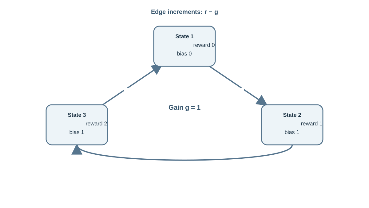
Take a three-state chain with a single action and fixed transitions. State 1 goes to state 2. State 2 goes to state 3. State 3 goes back to state 1. Rewards are , , .
The chain is a single cycle, so it is unichain and the gain is the average reward per step:
Now solve the bias equations. With one action, the Bellman relationship is :
These are consistent but underdetermined, as expected. Fix the reference . Then and .
| State | Reward | Gain | Bias |
|---|---|---|---|
| 1 | 0 | 1 | 0 |
| 2 | 1 | 1 | 1 |
| 3 | 2 | 1 | 1 |
Verify by plugging back in. For state 2: . For state 3: . Both hold.
Notice what the bias values are not. They are not rewards, and they are not discounted values. They measure transient advantage relative to the long-run rate. State 1 has zero immediate reward and the lowest bias, because it sits one step from the high-reward region. States 2 and 3 carry the same bias even though their rewards differ, because each is one step from the same successor structure. Two states with different immediate reward can carry identical bias for exactly that reason.
Knowledge check
Check your understanding
Answer this question before you continue.
What Gain and Bias Actually Tell You
Gain is the long-run reward rate the policy sustains. It is the quantity average-reward control optimizes.
Bias is the transient offset from that rate. Once the rate is fixed, bias decides which states are worth being in.
Two mistakes show up constantly.
Common mistake: Treating bias as a value function and comparing bias magnitudes across different policies. The additive constant makes that comparison meaningless. Two policies can have identical behavior and bias vectors that differ by a constant.
Common mistake: Assuming the gain is state-independent without checking the unichain condition. If the chain has two recurrent classes, the agent's long-run rate depends on where it starts, and the single-scalar formulation silently breaks.
The decision rule is short. If you care about steady-state throughput, cost per step, or uptime, optimize gain. If you care about reaching a goal or about near-term reward, the discounted or episodic formulation fits better.
Assumptions, Failure Modes, and When to Use This
Unichain is the load-bearing assumption. Multichain MDPs require a state-dependent gain or a more elaborate formulation, and the clean derivation above does not apply.
Average-reward algorithms usually need to estimate the gain online. That adds a moving target to the update and complicates convergence reasoning compared with the discounted contraction argument. Relative value iteration and related methods exist precisely because the plain Bellman operator is not a contraction in the average-reward setting.
When not to use this:
- Episodic tasks with natural termination.
- Tasks where near-term reward genuinely matters more.
- Settings where you cannot assume a single recurrent class.
Where it earns its place: inventory management, admission control, and other continuing operational problems with no reset and no reason to prefer reward now over reward later.
Where to Go Next
Turn the derivation into a decision rule. Check whether the task terminates. Check whether time preference is real. Check whether the induced chain is unichain. If the task continues and you care about steady-state rate, the average-reward Bellman relationship is the right formal object, and gain and bias are the two quantities to track.
The next practical step is to implement a relative value iteration loop on the three-state chain above. Watch the gain estimate settle toward 1 while the bias values shift by a constant. That shift is the additive-constant freedom made visible, and seeing it once will keep you from misreading bias as a value function later.
Knowledge check
Final check
Finish the article by checking the ideas you just learned.
References
Build a stronger RL mental model
Use structured resources to connect equations, algorithms, and observable agent behavior.


