Deriving Bellman Equations and Value Updates With a Worked Example

You can read $V(s) = R + \gamma V(s')$ a hundred times and still freeze when a variant shows up with a max, an expectation, or a $Q$ instead of a $V$. The formula is not the hard part. The hard part is that nobody showed you where it came from.

So let's derive it. We start from the definition of return, take one step of algebra at a time, and finish with a number you can check on paper. If you already have the intuition that value predicts future reward and that a Bellman relationship is one-step reward plus discounted continuation, you have everything you need. This article shows where that structure is forced to exist.

What You Need Before the Derivation

A derivation with hidden steps is just a formula wearing a costume. So we set up notation and assumptions first, and we name what breaks when they fail.

The return $G_t$ is the discounted sum of everything the agent collects from time step $t$ onward:

$G_t = R_{t+1} + \gamma R_{t+2} + \gamma^2 R_{t+3} + \cdots$

That definition hides the single most useful fact in this whole article. Factor out the first term:

$G_t = R_{t+1} + \gamma \left( R_{t+2} + \gamma R_{t+3} + \cdots \right) = R_{t+1} + \gamma G_{t+1}$

This one line is the engine. Everything else is bookkeeping.

Two assumptions make the recursion valid. First, the Markov property: the next state and reward depend only on the current state and action, not on the history that produced them. Second, either the task is episodic with terminal states that end the sum, or it is continuing with $\gamma < 1$ so the infinite sum stays finite under bounded rewards.

Warning: These are standard sufficient conditions, not universal laws. If your state representation is not Markov, the recursion breaks for that state variable — but you can repair it by augmenting the state with the missing history. And $\gamma = 1$ in a continuing task does not automatically diverge; finiteness depends on the reward structure and the task itself. The safe default is $\gamma < 1$ with bounded rewards.

From Return to the Bellman Expectation Equation

The state value under policy $\pi$ is the expected return starting from $s$:

$V^\pi(s) = \mathbb{E}\left[ G_t \mid S_t = s \right]$

Substitute the recursive identity for $G_t$:

$V^\pi(s) = \mathbb{E}\left[ R_{t+1} + \gamma G_{t+1} \mid S_t = s \right]$

Expectation is linear, so split it:

$V^\pi(s) = \mathbb{E}\left[ R_{t+1} \mid S_t = s \right] + \gamma \, \mathbb{E}\left[ G_{t+1} \mid S_t = s \right]$

Now expand each expectation over the two sources of randomness: the policy chooses $a$, then the environment chooses $s'$. The first term becomes a sum over actions and next states weighted by their probabilities. The second term is the key move — the expected return from the next state is exactly $V^\pi(s')$ by definition:

$V^\pi(s) = \sum_a \pi(a \mid s) \sum_{s'} P(s' \mid s, a) \left[ R(s, a) + \gamma V^\pi(s') \right]$

That is the Bellman expectation equation. Notice what happened: the unknown $V^\pi$ appears on both sides. The equation is self-referential, which is what makes it a Bellman equation rather than a plain sum.

The action value follows the same logic, except the first action is fixed rather than sampled from the policy:

$Q^\pi(s, a) = R(s, a) + \gamma \sum_{s'} P(s' \mid s, a) \, V^\pi(s')$

And the two quantities bridge into each other. Average $Q$ over the policy's action choices and you recover $V$:

$V^\pi(s) = \sum_a \pi(a \mid s) \, Q^\pi(s, a)$

Note: The expectation equation is a consistency condition, not an algorithm. It says what the values must satisfy. It does not say how to find them.

Where the Max Comes From: The Bellman Optimality Equation

The expectation equation describes a fixed policy. The optimality equation describes the best policy available, and the difference between them is one operator.

Define $V^*(s)$ as the best return achievable from $s$ over all policies, and $Q^*(s, a)$ as the best return when you commit to action $a$ first and then act optimally forever after.

The argument is short. From state $s$, the first action is yours to choose. Everything after that is, by definition, optimal. So you pick the action that maximizes immediate reward plus discounted optimal continuation:

$V^*(s) = \max_a \left[ R(s, a) + \gamma \sum_{s'} P(s' \mid s, a) \, V^*(s') \right]$

For action values, the max moves one step later, because the first action is already fixed:

$Q^*(s, a) = R(s, a) + \gamma \sum_{s'} P(s' \mid s, a) \max_{a'} Q^*(s', a')$

Put the two families side by side:

Same skeleton, one operator swapped. Once you have $Q^*$, the optimal policy is greedy with respect to it: $a^*(s) = \arg\max_a Q^*(s, a)$.

Common mistake: Treating the optimality equation as a method. It assumes you can evaluate every action in every state. When the model is unknown, the equation tells you the target but not how to reach it.

A Worked Value Update You Can Check by Hand

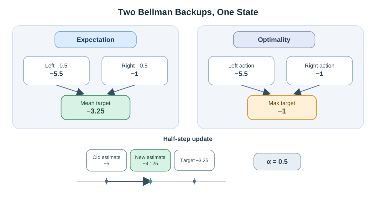
Theory earns trust when the arithmetic agrees. Here is a two-state setup small enough to verify with a calculator.

State A has two actions. Left stays in A. Right moves to terminal state B. Every transition gives a reward of $-1$, transitions are deterministic, and $\gamma = 0.9$. The policy is a coin flip: $\pi(\text{left} \mid A) = 0.5$ and $\pi(\text{right} \mid A) = 0.5$. Suppose the current estimate is $V(A) = -5$.

Expectation backup. Plug the current estimate into the right-hand side of the expectation equation. This evaluated right-hand side is the backup target, written $T^\pi V(A)$:

$T^\pi V(A) = 0.5 \left[ -1 + 0.9 \cdot V(A) \right] + 0.5 \left[ -1 + 0.9 \cdot 0 \right]$

The right branch ends at a terminal state, so it contributes no continuation term — that is why the recursion bottoms out. Evaluate:

$T^\pi V(A) = 0.5(-1 - 4.5) + 0.5(-1) = -2.75 - 0.5 = -3.25$

This is not the true value $V^\pi(A)$. It is the one-step target computed from the current estimate. The true value is the fixed point where the estimate equals its own backup — a different number that you would reach only after many sweeps.

Optimality backup. Same state, but now the agent picks the better action:

$T^* V(A) = \max\left[ -1 + 0.9 \cdot V(A), \; -1 + 0.9 \cdot 0 \right] = \max(-5.5, \; -1) = -1$

The difference between $-3.25$ and $-1$ is the max. The expectation equation averages the two branches; the optimality equation refuses the worse one.

The update. In practice you rarely jump straight to the target. You move toward it:

$\text{new estimate} = \text{old estimate} + \alpha \left( \text{target} - \text{old estimate} \right)$

With $\alpha = 0.5$ and the expectation target, the new estimate is $-5 + 0.5(-3.25 - (-5)) = -4.125$. The estimate moves toward the target. Repeat the sweep and it keeps moving, converging to the fixed point of the expectation equation — not to $-3.25$ in one step.

A backup diagram makes the flow visible: open circles for states, filled circles for state-action pairs, lines for actions and transitions. Values flow backward from $s'$ into $s$ along those lines.

What the Derivation Buys You

The equations are the reason dynamic programming, TD learning, and Q-learning look like relatives. Each one approximates the same fixed-point condition and substitutes something different for the expectation.

When you know the model — $P$ and $R$ — you can sweep the equations directly. When you do not, you replace the expectation with a sampled transition and get a stochastic update. The expectation equation is the target for policy evaluation; the optimality equation is the target for control. That is the prediction/control split written as algebra.

Common mistake: Treating the Bellman equation as a definition of value rather than a constraint value must satisfy. Early in training, estimates are wrong. The equation is not broken — your estimate has not converged to it yet.

And know when not to lean on these equations: large or continuous state spaces where exact sweeps are impossible, and settings where your state representation violates the Markov property.

When you meet a new value-based algorithm, ask two questions. Which Bellman relationship is it approximating? And what does it substitute for the expectation — a model, a sample, or a learned critic? Those two answers tell you more about the method than its name does.

Your next move: close this article and re-derive the optimality equation from memory on the two-state example above. If the max lands in the right place without looking, you own the derivation. If it does not, you now know exactly which line to re-read.