Implement Policy Evaluation and Value Iteration for a Small MDP

The Bellman equation looks like a definition. It is really a loop you can run.

That distinction matters. You can read about backups for an hour and still not trust them. The moment you watch a value estimate move — one number, one state, one sweep — the equation stops being notation and becomes a tool. So we will build the smallest thing that produces that moment: one tiny MDP, two functions, and printed output you can check with a calculator.

By the end you will have a converged value table, a greedy policy, and a hand-verified number. That last part is the one most tutorials skip, and it is the one that tells you whether you actually understood the code or just ran it.

What You Are Actually Building

This is planning on a known MDP. You are handed the transition probabilities and rewards up front. Nothing is learned from experience, no agent wanders around collecting samples. You already know the map; you are computing the best route.

Two functions do the work:

• Iterative policy evaluation — given a fixed policy, compute the value of every state under it. This is an expectation backup.
• Value iteration — compute the optimal values directly, no policy required. This is a max backup.

The only structural difference between them is expectation versus maximum. Everything else — the sweep, the delta, the stopping threshold — is identical. If you have read how Bellman backups decompose a value into one-step reward plus a discounted continuation estimate, this article is where that idea becomes a for-loop.

Assumptions and setup:

• Python 3. No NumPy required, though you can swap it in later.
• No external services, no credentials, no downloads.
• Runs in well under a second.

Success criteria, stated now so you know when you are done: a value table that stops changing, a greedy policy extracted from it, and at least one state value you verified by hand against the Bellman equation.

The Tiny MDP We Will Solve

Four states, two actions, one terminal state, and a small penalty for every step that is not terminal. Small enough to draw on paper, which is the point — every number later has a traceable source.

States: S0, S1, S2, S3. S3 is terminal. Actions: left, right.

The step penalty is -1 for any transition that does not land in S3, and 0 for transitions that do. This is the classic "reach the goal, pay for every step" setup: the agent wants the shortest path.

We will write the model as plain dictionaries. No framework, no hidden abstraction.

import math

STATES = ["S0", "S1", "S2", "S3"]
ACTIONS = ["left", "right"]
TERMINAL = "S3"
GAMMA = 0.9

# transitions[(state, action)] = list of (probability, next_state)
TRANSITIONS = {
    ("S0", "left"):  [(1.0, "S0")],
    ("S0", "right"): [(1.0, "S1")],
    ("S1", "left"):  [(1.0, "S0")],
    ("S1", "right"): [(1.0, "S2")],
    ("S2", "left"):  [(1.0, "S1")],
    ("S2", "right"): [(1.0, "S3")],
    ("S3", "left"):  [(1.0, "S3")],
    ("S3", "right"): [(1.0, "S3")],
}

def reward(state, action, next_state):
    return 0.0 if next_state == TERMINAL else -1.0

The transitions here are deterministic, which keeps the arithmetic checkable by hand. The code does not care — it sums over a probability list, so you can make any transition stochastic later by splitting the probability.

A note on GAMMA = 0.9. The discount factor controls how much future reward counts today. Values near 1 make distant rewards matter more, which makes values larger and convergence slower. Values near 0 make the agent short-sighted. I pick 0.9 here because it is far enough from 1 to converge quickly and far enough from 0 to make the continuation term visible in the numbers.

The assumptions we are using: finite states, finite actions, stationary transitions (the probabilities do not change over time), and a discounted episodic setting with a terminal state.

One Backup by Hand Before Any Loop

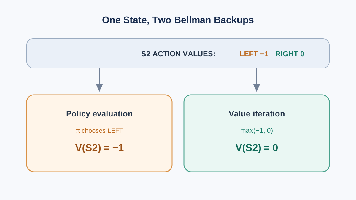
Before writing a loop, do one backup on one state. This is the drill. If you can do this, the algorithm is just a for loop around it.

Take S2 with the action right. The transition is deterministic to S3. Suppose our current estimate for every state is 0. The backup is:

expected value of (S2, right)
  = sum over next states of  P(next) * ( reward + GAMMA * V(next) )
  = 1.0 * ( 0 + 0.9 * V(S3) )
  = 1.0 * ( 0 + 0.9 * 0 )
  = 0

Now the same state with left, which goes to S1:

expected value of (S2, left)
  = 1.0 * ( -1 + 0.9 * V(S1) )
  = 1.0 * ( -1 + 0.9 * 0 )
  = -1

The max version of the backup takes the larger of these: max(0, -1) = 0. So after one value-iteration backup, V(S2) becomes 0. The expectation version, given a policy that picks left in S2, would set V(S2) to -1.

Same arithmetic. One takes an average weighted by the policy; the other takes the best action. That is the entire difference between the two algorithms you are about to write.

Tip: Print the before and after value for a single state on the first sweep. Watching -1 become 0 is worth more than reading the equation three more times.

Policy Evaluation in Code

Policy evaluation answers one question: if the agent follows this policy forever, what is each state worth?

Define the policy as a dictionary from state to action. That makes the expectation explicit — for each state, you look up the action, then sum over the transitions for that action.

def policy_evaluation(policy, theta=1e-6, max_sweeps=1000):
    V = {s: 0.0 for s in STATES}
    for sweep in range(max_sweeps):
        delta = 0.0
        for s in STATES:
            v_old = V[s]
            a = policy[s]
            v_new = 0.0
            for prob, s_next in TRANSITIONS[(s, a)]:
                v_new += prob * (reward(s, a, s_next) + GAMMA * V[s_next])
            V[s] = v_new
            delta = max(delta, abs(v_old - v_new))
        if sweep % 5 == 0:
            print(f"sweep {sweep:3d}  delta={delta:.6f}  V={ {k: round(v,4) for k,v in V.items()} }")
        if delta < theta:
            print(f"converged after {sweep + 1} sweeps")
            break
    return V

Two details carry the weight here.

First, delta is the largest single-state change in the sweep, not the total change. If one state moved by 0.4 and nine states moved by 0.001, delta is 0.4. That is the right signal: the loop is only done when no state is still moving.

Second, the update is in place — V[s] is overwritten as we go, so later states in the same sweep see the fresh value. This is called a Gauss-Seidel sweep, and it usually converges faster than updating into a separate array. It is also slightly harder to reason about, which is why the debugging section below covers the two-array alternative.

Run it with a policy that always goes right:

policy = {s: "right" for s in STATES}
V_pi = policy_evaluation(policy)

Expected output: values climb from 0 toward their fixed point, delta shrinks each sweep, and the loop stops when delta < 1e-6. The terminal state stays at 0 because its reward is 0 and it transitions to itself.

Value Iteration in Code

Now change one line. Replace the policy lookup with a max over actions.

def value_iteration(theta=1e-6, max_sweeps=1000):
    V = {s: 0.0 for s in STATES}
    for sweep in range(max_sweeps):
        delta = 0.0
        for s in STATES:
            v_old = V[s]
            best = -math.inf
            for a in ACTIONS:
                q = 0.0
                for prob, s_next in TRANSITIONS[(s, a)]:
                    q += prob * (reward(s, a, s_next) + GAMMA * V[s_next])
                best = max(best, q)
            V[s] = best
            delta = max(delta, abs(v_old - V[s]))
        if delta < theta:
            print(f"value iteration converged after {sweep + 1} sweeps")
            break
    return V

That is the whole algorithm. The sweep structure, the delta accumulator, and the threshold are identical to policy evaluation. The only change is best = max(best, q) instead of a single policy-weighted sum.

Why does this not need a policy to start? Because it is implicitly improving the greedy policy at every sweep. Each backup asks "what if I take the best action here, assuming my current estimates are right?" The estimates get better, the implied policy gets better, and the two chase each other to a fixed point.

Extract the greedy policy once values have converged:

def greedy_policy(V):
    policy = {}
    for s in STATES:
        best_a, best_q = None, -math.inf
        for a in ACTIONS:
            q = sum(prob * (reward(s, a, s_next) + GAMMA * V[s_next])
                    for prob, s_next in TRANSITIONS[(s, a)])
            if q > best_q:
                best_a, best_q = a, q
        policy[s] = best_a
    return policy

V_star = value_iteration()
pi_star = greedy_policy(V_star)
for s in STATES:
    print(f"{s}: V*={V_star[s]:.4f}  pi*={pi_star[s]}")

Expected output: S0 and S1 both point right, S2 points right, and S3 is arbitrary because it is terminal. The optimal values decrease as you move away from the terminal state, which is exactly what a step penalty should produce.

Note: A small theta can still yield the optimal policy even when values are slightly off. The greedy choice only flips when two actions are nearly tied, so a "close enough" value table often produces the exact optimal policy.

Checking the Numbers Instead of Trusting Them

Printed output is not evidence until you verify it. Here are the checks I run every time.

Hand-check one state. Take the converged values and plug S2 back into the Bellman equation. With GAMMA = 0.9 and V(S3) = 0, the value of going right from S2 is 0 + 0.9 * 0 = 0. The value of going left is -1 + 0.9 * V(S1). If V(S1) is around -1.9, then left gives roughly -2.71, which is worse. So V(S2) should be 0. If your printed value is not 0, something upstream is wrong.

Sanity checks. The terminal state value should be 0. Values should be monotone in distance from the terminal state under a step penalty — farther states are worth less. If S0 is worth more than S1, your transition table is probably reversed.

Compare against the fixed policy. The optimal values should dominate the evaluated policy values state by state. If V_pi[S0] > V_star[S0], you have a bug, because the optimal policy is by definition at least as good as any fixed policy.

What a wrong answer looks like. Values that oscillate, grow without bound, or sit at zero usually mean one of three things: a transition list that does not sum to 1.0, a reward applied to the wrong state, or GAMMA = 1.0 in a non-terminating MDP.

Failure Modes and Debugging Signals

Transition probabilities that do not sum to one. This is the most common silent bug. Add a check:

for (s, a), outcomes in TRANSITIONS.items():
    total = sum(p for p, _ in outcomes)
    assert abs(total - 1.0) < 1e-9, f"{s},{a} sums to {total}"

Reward indexed by the wrong thing. You can define reward as R(s, a, s') or as R(s'). Pick one convention and stay consistent. Mixing them produces values that look plausible but are quietly wrong.

GAMMA = 1.0 in a non-terminating MDP. Values grow without bound and the loop never converges. Discounting is what guarantees the fixed point exists in the infinite-horizon case.

theta too large. The loop stops early and can produce a suboptimal greedy policy. Start with 1e-6 and only loosen it if you have a reason.

In-place versus two-array updates. The code above updates V in place. The two-array version writes into a fresh V_new and swaps at the end of the sweep. Two-array is easier to reason about because every state in a sweep sees the same snapshot; in-place is usually faster. If your values behave strangely, switch to two-array and see whether the behavior changes. If it does, you were relying on update order.

One Experiment Worth Running

The most instructive parameter to sweep is GAMMA. Run value iteration for GAMMA in [0.5, 0.9, 0.99] and record the number of sweeps and the final value of S0.

You will see two things. Higher GAMMA makes values larger, because distant rewards count more. And higher GAMMA makes convergence slower, because each backup shrinks the distance to the true value by roughly the discount factor. At 0.5, the correction is aggressive and the loop finishes fast. At 0.99, each sweep barely moves the estimate.

Print V(S0) after every sweep and watch the correction curve flatten. That flattening is the fixed-point behavior in action — the same mechanism that makes Bellman updates converge at all.

Then sweep theta across [1e-2, 1e-4, 1e-6] and watch the tradeoff between iteration count and value accuracy. You will usually find that the greedy policy stabilizes well before the values do.

Where This Leaves You

The decision rule to carry forward: when you have a known model and a small state space, write the transition table as plain data, run one backup by hand, then loop it. Verify one state against the Bellman equation before you trust the rest. The code is short; the verification is what makes it real.

From here, the natural next step is policy iteration — alternate a full evaluation with a greedy improvement step and watch the policy stabilize in a handful of rounds. The other direction is the model-free setting, where the transition table is no longer given and you have to estimate values from sampled experience instead. Same Bellman logic, less information, more noise.