Deriving the Policy Improvement Theorem for Tabular MDPs

You run a round of policy iteration. The greedy policy looks better on paper, so you deploy it. The measured return drops. Nothing in your code threw an error, and nothing in the textbook was wrong. What broke was the mental model you were carrying: the belief that greedy improvement is always an improvement. It is not. It is an improvement if a specific set of conditions holds. This article derives the policy improvement theorem for tabular MDPs, names those conditions, and shows exactly where the guarantee leaks when you replace exact values with estimates.

What the Theorem Actually Claims

Before the derivation, state the result precisely. Let $\pi$ and $\pi'$ be deterministic policies over a finite MDP. If, for every state $s$,

$Q^{\pi}(s, \pi'(s)) \geq V^{\pi}(s),$

then

$V^{\pi'}(s) \geq V^{\pi}(s) \quad \text{for all } s.$

Read the hypothesis carefully. It is a per-state, pointwise comparison: at each state, the action $\pi'$ picks must be worth at least as much as the current policy's value there. This is stronger than "better on average." A policy that improves the average return while quietly regressing in a few states does not satisfy the hypothesis, and the theorem says nothing about it.

Greedy improvement is the special case where $\pi'(s) = \arg\max_a Q^{\pi}(s, a)$. Since the max is at least the policy-weighted average, the hypothesis holds automatically — provided you have the true $Q^{\pi}$.

Two things the theorem does not say:

• It does not promise strict improvement. Ties are allowed, and the conclusion is $\geq$, not $>$.
• It does not say the greedy policy is optimal after one step. Optimality requires the full policy iteration loop plus Bellman optimality.

If you already have the Bellman expectation relationship from the prerequisite material, you have everything you need. The only tool this proof uses is the one-step decomposition: value equals expected immediate reward plus discounted expected next-state value.

Notation and the Assumptions That Carry the Proof

Here is the notation used throughout, with each symbol tied to what it represents in the system.

I use the deterministic-policy convention in the greedy step: $\pi'(s)$ denotes the single action $\pi'$ selects at $s$. This keeps the algebra readable. The result extends to stochastic policies, but the deterministic case is where the intuition lives.

Four assumptions carry the proof:

1. Finite tabular MDP with exact evaluation. The proof compares against true action values $Q^{\pi}$, not estimates. This is the assumption that breaks most often in practice.
2. Discounting regime. $\gamma < 1$ for continuing tasks. For $\gamma = 1$, the theorem holds only when trajectories terminate in bounded time — episodic structure with a finite horizon.
3. Rich enough policy class. The policy class must be able to represent the greedy choice at every state. Deterministic policies over the full action set satisfy this.
4. Stationary environment and the Markov property. $Q^{\pi}$ must be a well-defined function of state and action alone.

Keep these four in view. They are the same four things that fail when a real algorithm misbehaves.

Deriving the Inequality Step by Step

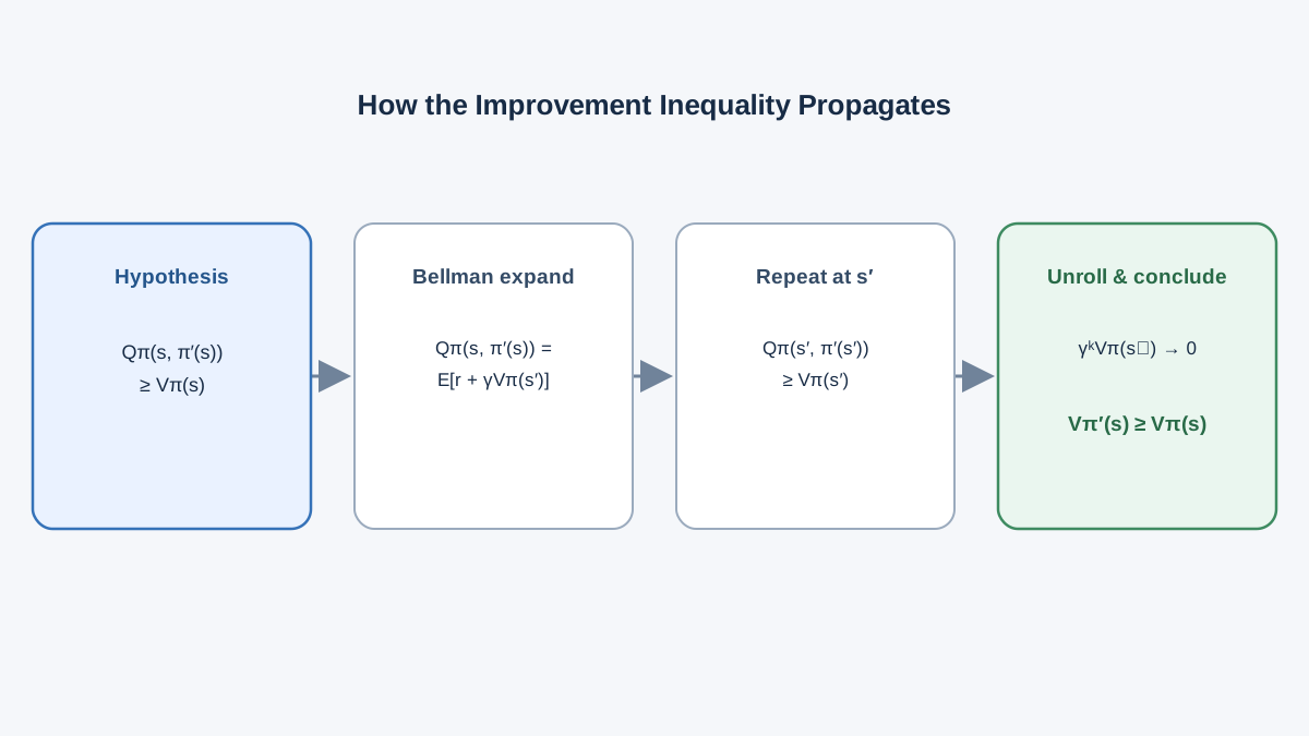
The proof is a chain of substitutions, and every line has a reason. Follow the reasons, not the symbols.

Step 1 — Value as a policy-weighted average.

$V^{\pi}(s) = \sum_a \pi(a \mid s) \, Q^{\pi}(s, a).$

This is just the definition: the value of a state under $\pi$ is the average of the action values, weighted by how often $\pi$ picks each action.

Step 2 — Apply the hypothesis directly.

The theorem's hypothesis gives us $Q^{\pi}(s, \pi'(s)) \geq V^{\pi}(s)$ at every state. That is the inequality we need — no maximization required. Substituting the definition from Step 1:

$V^{\pi}(s) = \sum_a \pi(a \mid s) Q^{\pi}(s, a) \leq Q^{\pi}(s, \pi'(s)).$

The left side is the current policy's value; the right side is the value of the action $\pi'$ selects. The hypothesis is what licenses the step. If $\pi'$ happens to be greedy, the inequality is tight at the max; if $\pi'$ merely matches or beats the average, the inequality still holds.

Step 3 — Expand the action value.

$Q^{\pi}(s, \pi'(s)) = \mathbb{E}_{\pi'}\!\left[\, r_{t+1} + \gamma V^{\pi}(s_{t+1}) \,\middle|\, s_t = s \,\right].$

The immediate reward is taken under $\pi'$'s action, but the continuation is still valued under $\pi$. This mismatch is the whole point — it is what we are about to repair.

Step 4 — Apply the same inequality at the next state.

At $s_{t+1}$, the hypothesis gives $V^{\pi}(s_{t+1}) \leq Q^{\pi}(s_{t+1}, \pi'(s_{t+1}))$. Substituting:

$V^{\pi}(s) \leq \mathbb{E}_{\pi'}\!\left[\, r_{t+1} + \gamma Q^{\pi}(s_{t+1}, \pi'(s_{t+1})) \,\middle|\, s_t = s \,\right].$

Expand the inner $Q^{\pi}$ the same way and repeat:

$V^{\pi}(s) \leq \mathbb{E}_{\pi'}\!\left[\, r_{t+1} + \gamma r_{t+2} + \gamma^2 V^{\pi}(s_{t+2}) \,\middle|\, s_t = s \,\right].$

This is the unrolling step. The guarantee is earned here. Each state's improvement is paid forward to its successors, and the inequality survives every substitution because it held at every state.

Step 5 — Take the limit.

After $k$ unrollings:

$V^{\pi}(s) \leq \mathbb{E}_{\pi'}\!\left[\, \sum_{j=0}^{k-1} \gamma^j r_{t+j+1} + \gamma^k V^{\pi}(s_{t+k}) \,\middle|\, s_t = s \,\right].$

As $k \to \infty$, the residual term $\gamma^k V^{\pi}(s_{t+k})$ vanishes when $\gamma < 1$, because $V^{\pi}$ is bounded and $\gamma^k \to 0$. For episodic tasks with $\gamma = 1$, the residual vanishes once trajectories terminate. What remains is exactly $V^{\pi'}(s)$. The conclusion follows.

The proof is a bootstrap argument. Improvement at one state is not free — it is collateralized by improvement at its successors. If any successor refuses to improve, the chain of inequalities snaps.

Worked Example: One Improvement Step on a Tiny MDP

Two states, two actions, $\gamma = 0.9$. From state $s_1$, action $a$ transitions to $s_2$ with reward $1$; action $b$ stays in $s_1$ with reward $0$. From $s_2$, both actions stay in $s_2$ with reward $0$. Start with $\pi$: always take $b$ in $s_1$, always take $a$ in $s_2$.

Evaluate $\pi$. From $s_1$, the agent loops forever taking $b$ with reward $0$, so $V^{\pi}(s_1) = 0$. From $s_2$, same story: $V^{\pi}(s_2) = 0$.

Compute action values at $s_1$:

• $Q^{\pi}(s_1, a) = 1 + 0.9 \cdot V^{\pi}(s_2) = 1$
• $Q^{\pi}(s_1, b) = 0 + 0.9 \cdot V^{\pi}(s_1) = 0$

The greedy policy $\pi'$ takes $a$ at $s_1$. Check the hypothesis: $Q^{\pi}(s_1, \pi'(s_1)) = 1 \geq V^{\pi}(s_1) = 0$. Holds. At $s_2$, both actions tie at $0$, so the inequality is tight — a live demonstration that "at least as good" is not a formality.

Now evaluate $\pi'$. From $s_1$: reward $1$, then $s_2$ forever with reward $0$, so $V^{\pi'}(s_1) = 1$. From $s_2$: $V^{\pi'}(s_2) = 0$. The conclusion holds: $1 \geq 0$ and $0 \geq 0$.

Run this by hand. Change one reward. Watch which inequality breaks first.

Where the Guarantee Comes From — and Where It Leaks

In the exact case, policy iteration with full evaluation converges to an optimal policy. The theorem plus Bellman optimality is what makes the loop terminate: each improvement step is monotone, and a finite MDP has finitely many deterministic policies, so the sequence must stabilize at a policy that is greedy with respect to its own value function — an optimal one.

The approximate case is where the guarantee leaks. When $Q^{\pi}$ is estimated from samples or a function approximator, the greedy step is taken against noisy values. The hypothesis $Q^{\pi}(s, \pi'(s)) \geq V^{\pi}(s)$ may be false at some states, and the proof's chain of inequalities has nothing to stand on. Approximate policy evaluation gives you a heuristic improvement step, not a monotonic guarantee. Measured return can regress.

Common mistake: Assuming the theorem licenses "always take the argmax of my current Q estimate" in deep RL or with limited data. The theorem licenses that step only when the estimate is the true $Q^{\pi}$.

This is why conservative improvement methods exist — trust regions, small step sizes, statistical lower bounds on the new policy's performance. They are not refinements of the theorem. They are replacements for a guarantee that is no longer available.

One boundary worth stating explicitly: the theorem also fails for episodic tasks with $\gamma = 1$ if some trajectories never terminate. A policy can look greedy against optimal action values and still be terrible, because the residual term never vanishes. The discount factor is not a tuning knob here. It is a load-bearing assumption.

What to Check Before You Trust an Improvement Step

Turn the derivation into a checklist:

• Is your $Q$ estimate exact or sampled? If sampled, treat the improvement as a hypothesis to test, not a guarantee.
• Is your discounting regime inside the theorem's scope? $\gamma < 1$, or episodic with bounded trajectories.
• Are you comparing per-state values, or only aggregate return? Aggregate improvement can hide per-state regressions.
• Does your policy class actually contain the greedy choice, or are you approximating it?

My rule: use the theorem to reason about the shape of the algorithm. Use measured evaluation to decide whether a specific update helped. The theorem tells you what must be true for greedy improvement to be safe. That list of conditions is the same list of things that break in practice.

Here is your next experiment. Take the two-state example above. Replace the exact $Q^{\pi}$ values with noisy estimates — add a small random perturbation to each. Run the greedy step. Compute the true $V^{\pi'}$ and compare it to $V^{\pi}$. Repeat a hundred times and count how often the guarantee fails. You will not need a proof to remember the lesson after that.