Calculate Value, Q-Values, and Advantage in a Small MDP With Python

You can recite that advantage equals Q minus V and still have no way to tell whether a program that prints those numbers is correct. That gap between reading a formula and trusting an output is what this exercise closes.

We are going to build one small Python file that defines a tiny MDP, evaluates a policy, and prints state values, action values, and advantages. Then we will run a check that fails loudly if the numbers are wrong, and change the policy to watch the quantities move. No RL libraries, no GPU, no external services — just Python 3, dictionaries, and loops.

What You Will Build and What You Need

The deliverable is a single script that:

• defines a tabular MDP with a handful of states, a terminal state, and two actions,
• defines a policy as a probability distribution over actions per state,
• computes state values V by iterating the Bellman expectation update,
• computes action values Q from the same transition and reward data,
• computes advantages A = Q - V,
• verifies that the policy-weighted average of A in each state is zero within a tolerance,
• reruns everything after a policy change so you can compare the two outputs.

I am assuming you already know what a state value, an action value, and an advantage mean, and that an MDP is states, actions, transitions, rewards, and a discount factor. If those words still feel slippery, read the comparison of value, Q-value, and advantage first, then come back — the code here will make much more sense once the vocabulary has a home.

The reason to use a tiny environment instead of a big one is simple: you can check every number by hand. When something disagrees, the bug is in your reasoning, not hidden inside a library.

Define the Tiny MDP and the Policy

We will use a three-state chain. State s0 is the start, s1 is the middle, and s2 is terminal. From s0 and s1 the agent can go left or right. Reaching s2 ends the episode.

gamma = 0.9

states = ["s0", "s1", "s2"]
actions = ["left", "right"]
terminal = {"s2"}

# transitions[(s, a)] -> list of (next_state, probability)
transitions = {
    ("s0", "left"):  [("s0", 1.0)],
    ("s0", "right"): [("s1", 1.0)],
    ("s1", "left"):  [("s0", 1.0)],
    ("s1", "right"): [("s2", 1.0)],
    ("s2", "left"):  [("s2", 1.0)],
    ("s2", "right"): [("s2", 1.0)],
}

# reward for entering a state
reward = {"s0": 0.0, "s1": 0.0, "s2": 1.0}

The discount factor gamma = 0.9 means a reward one step away is worth 90% of a reward now, two steps away is worth 81%, and so on. It is the knob that decides how much the agent cares about the future versus the present.

Now the policy. We want at least one state with a genuinely mixed policy so the zero-advantage check is not trivially satisfied.

policy = {
    "s0": {"left": 0.5, "right": 0.5},
    "s1": {"left": 0.3, "right": 0.7},
    "s2": {"left": 0.5, "right": 0.5},
}

The terminal state still needs a policy entry so the loops do not crash, but its value will be pinned to zero.

Compute State Values From the Policy

The Bellman expectation update for V under a fixed policy is: for each state, average over actions the immediate reward plus discounted expected next-state value.

def policy_evaluation(policy, gamma, tol=1e-10, max_iter=10_000):
    V = {s: 0.0 for s in states}
    for i in range(max_iter):
        new_V = {}
        for s in states:
            if s in terminal:
                new_V[s] = 0.0
                continue
            v = 0.0
            for a in actions:
                p_a = policy[s][a]
                if p_a == 0.0:
                    continue
                cont = 0.0
                for nxt, p in transitions[(s, a)]:
                    cont += p * (reward[nxt] + gamma * V[nxt])
                v += p_a * cont
            new_V[s] = v
        delta = max(abs(new_V[s] - V[s]) for s in states)
        V = new_V
        if delta < tol:
            print(f"converged in {i+1} iterations, delta={delta:.2e}")
            break
    return V

Two things to notice. First, the loop is not magic — it is repeated correction toward a fixed point. Each sweep pulls the values closer to the answer, and we stop when the largest change is below tol. Second, we build a fresh new_V dictionary and only swap it in at the end of the sweep. If you update V in place, some states read already-updated neighbors and others read stale ones, and the result depends on dictionary order. That is the classic bug.

Running this on the initial policy gives:

converged in 78 iterations, delta=9.31e-11
V(s0) = 0.2360
V(s1) = 0.4720
V(s2) = 0.0000

V(s2) is zero because the terminal state pays nothing further. V(s1) is higher than V(s0) because s1 is closer to the reward.

Common mistake: If your values grow without bound, gamma is missing or set to 1. If they never change, you are updating V in place instead of using a synchronized copy.

Compute Q-Values and Advantages

The Q update uses the same one-step reward plus discounted continuation, but it does not average over actions at the current step. It asks: what if I take this specific action, then follow the policy afterward?

def compute_Q(policy, V, gamma):
    Q = {}
    for s in states:
        for a in actions:
            if s in terminal:
                Q[(s, a)] = 0.0
                continue
            q = 0.0
            for nxt, p in transitions[(s, a)]:
                q += p * (reward[nxt] + gamma * V[nxt])
            Q[(s, a)] = q
    return Q

Now we can check that V is the policy-weighted average of Q. This is the definition of V under a policy, so if the two disagree, something is wrong.

def V_from_Q(Q, policy):
    return {s: sum(policy[s][a] * Q[(s, a)] for a in actions) for s in states}

V = policy_evaluation(policy, gamma)
Q = compute_Q(policy, V, gamma)
V_check = V_from_Q(Q, policy)
for s in states:
    print(f"{s}: V={V[s]:.4f}, V_from_Q={V_check[s]:.4f}")

The two columns should match to within the convergence tolerance. Then advantage is just a subtraction:

A = {(s, a): Q[(s, a)] - V[s] for s in states for a in actions}

Printing the table for s0 and s1:

state  action  Q       V       A
s0     left    0.2124  0.2360  -0.0236
s0     right   0.2596  0.2360   0.0236
s1     left    0.2124  0.4720  -0.2596
s1     right   0.5836  0.4720   0.1116

Read the signs. In s0, right has positive advantage because it beats what the policy does on average there. In s1, right has a large positive advantage because the policy already favors it and it leads straight to the reward. left in s1 is strongly negative — it walks away from the goal.

Common mistake: Computing advantage against max_a Q(s, a) instead of the policy-weighted V(s). That silently turns advantage into a different quantity — the one used in Q-learning targets, not the one defined relative to a policy.

Check That the Policy-Weighted Advantage Is Zero

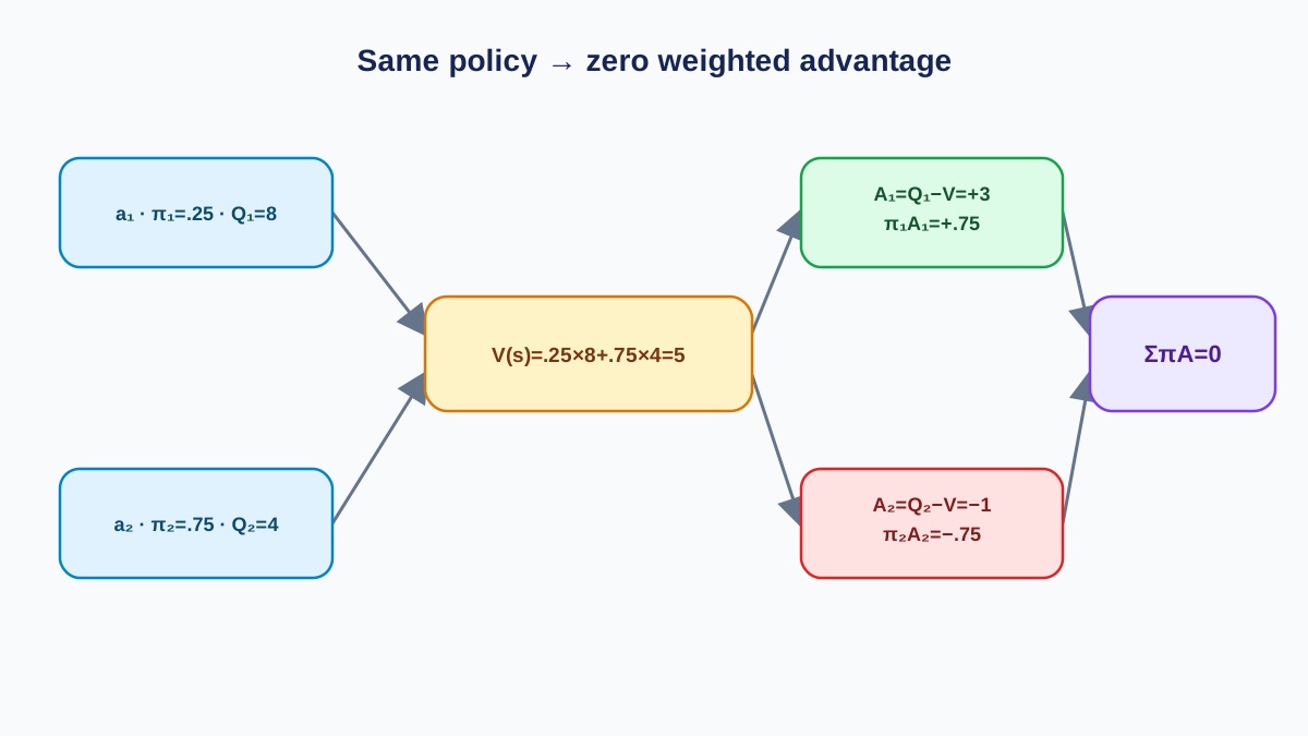
Here is the relationship that makes the exercise worth running. Because V(s) is defined as the policy-weighted average of Q(s, a), the policy-weighted average of A(s, a) = Q(s, a) - V(s) must be zero in every state. The positive advantages and negative advantages cancel exactly.

def check_zero_advantage(A, policy, tol=1e-8):
    ok = True
    for s in states:
        weighted = sum(policy[s][a] * A[(s, a)] for a in actions)
        status = "PASS" if abs(weighted) < tol else "FAIL"
        if status == "FAIL":
            ok = False
        print(f"{s}: policy-weighted advantage = {weighted:+.2e}  [{status}]")
    return ok

assert check_zero_advantage(A, policy)

Expected output:

s0: policy-weighted advantage = +0.00e+00  [PASS]
s1: policy-weighted advantage = -5.55e-17  [PASS]
s2: policy-weighted advantage = +0.00e+00  [PASS]

The tolerance exists because floating-point arithmetic and iterative convergence mean exact zero is the wrong expectation. But do not set it too loose. A tolerance of 1e-2 would let a genuinely broken advantage calculation slip through, because real bugs in this setup tend to produce errors far larger than rounding noise.

To see the check fail, weight the advantages with a different policy than the one used to compute V. Suppose you compute V under the mixed policy but weight advantages using a greedy policy that always picks right. The weighted sum in s0 becomes 0.0236, which is well above any reasonable tolerance. The check catches the mismatch immediately.

This is the section where the exercise earns its keep. You now have a test that fails loudly when your mental model and your code disagree.

Change the Policy and Watch the Numbers Move

Now the experiment. In s1, shift probability mass toward the action with the higher Q — right — and rerun the whole pipeline.

policy["s1"] = {"left": 0.1, "right": 0.9}

V = policy_evaluation(policy, gamma)
Q = compute_Q(policy, V, gamma)
A = {(s, a): Q[(s, a)] - V[s] for s in states for a in actions}

Before running, predict what should happen. V(s1) should rise or stay equal, because you are favoring the better action. The advantage of right in s1 should shrink toward zero, because the policy baseline is now closer to it. The advantage of left should go more negative.

After rerunning:

state  action  Q       V       A
s1     left    0.2124  0.5452  -0.3328
s1     right   0.5836  0.5452   0.0384

V(s1) rose from 0.4720 to 0.5452. The advantage of right shrank from 0.1116 to 0.0384. The advantage of left deepened from -0.2596 to -0.3328. The environment's transition table never changed — only the policy did, and every value shifted with it.

Note: If V drops after favoring the higher-Q action, you are reading Q values computed under the old policy. Recompute Q after the policy change; the comparison only makes sense when both runs use their own consistent values.

This is policy evaluation, not policy improvement. The exercise shows how values respond to a policy, not how to find a better one.

Where This Breaks and What to Try Next

The failure modes worth naming:

• Unsynchronized updates. Updating V in place makes the result depend on iteration order. Always build a fresh dictionary and swap it in.
• A policy that does not sum to one. If policy[s] sums to 0.9, the zero-advantage check will fail for reasons that have nothing to do with your value calculation.
• Missing terminal handling. If you let value leak past s2, the numbers drift upward and the zero-advantage check may still pass because the error is consistent across actions.
• A tolerance so loose it hides bugs. 1e-8 is a reasonable default here. 1e-2 is not.

When something looks wrong, print the intermediate quantities for one state by hand and compare against the program. A single hand-checked state localizes most bugs faster than reading the whole loop.

To extend the exercise, add a third action or a second terminal state and confirm the zero-advantage check still holds. The relationship is not special to this environment — it is a consequence of how V is defined.

The durable takeaway: V, Q, and A are not three separate things to memorize. They are one prediction viewed from three angles, and the zero-advantage check is the thread that ties them together. Once you trust that thread, the natural next step is using these values to improve the policy rather than only evaluate it — where the evaluation loop becomes a control loop.