
Explore Reward Ambiguity With a Tiny Inverse Reinforcement Learning Example
Two reward functions. One demonstrated path. No way to tell them apart from behavior alone.

Key topics
Two reward functions. One demonstrated path. No way to tell them apart from behavior alone.
That claim is easy to nod at and hard to feel. So let's build the smallest possible case where it happens, run it, and then break it on purpose.
The Task: One Path, Two Rewards
Here is the whole environment. A 2×3 grid:
S . .
. . G
The agent starts at S (top-left), wants to reach G (bottom-right), and can move up, down, left, or right. Moves that would leave the grid are illegal. Every step costs something; reaching G ends the episode.
The demonstration is one path:
S → (0,1) → (0,2) → (1,2)
Three moves. We treat this as the expert's optimal behavior.
To make "optimal" mean anything, we need an assumption. Ours is the standard one: the expert maximizes discounted return, the sum of rewards along the path, with each step's reward multiplied by γ^t for discount factor γ. I'll use γ = 0.9. Determinism matters here — no transition noise, no stochastic policy — so we can compute path preference exactly instead of estimating it.
If inverse RL is new to you, the short version: normal RL goes reward → behavior. Inverse RL goes behavior → reward. This exercise assumes that framing and jumps straight to the uncomfortable part — the mapping back is not unique.
Knowledge check
Check your understanding
Answer this question before you continue.
Two Reward Tables That Agree on the Path
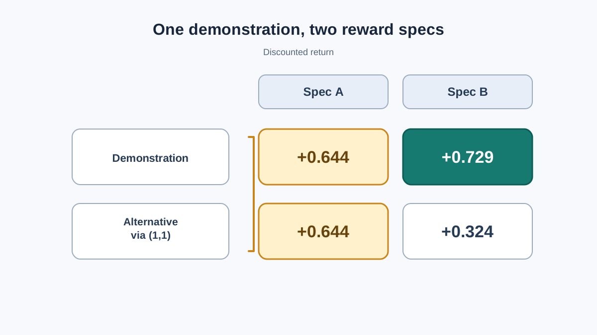
Here are two reward specifications. Both give +1 for reaching the goal.
Spec A — a small per-step cost:
| Event | Reward |
|---|---|
| Reach goal | +1 |
| Every other step | −0.05 |
Spec B — the same goal reward, but the penalty targets one specific state:
| Event | Reward |
|---|---|
| Reach goal | +1 |
Step into (1,1) | −0.5 |
| Every other non-goal step | 0 |
These are genuinely different functions. Spec A charges you for existing; Spec B charges you for one square. Neither is a rescaled copy of the other — you cannot multiply Spec A by a constant and get Spec B.
Now compute discounted returns by hand for the demonstrated path and one alternative.
Demonstrated path S → (0,1) → (0,2) → (1,2), rewards at steps 1–3:
- Spec A:
0.9(−0.05) + 0.81(−0.05) + 0.729(+1) ≈ 0.644 - Spec B:
0.9(0) + 0.81(0) + 0.729(+1) ≈ 0.729
Alternative path S → (1,0) → (1,1) → (1,2):
- Spec A:
0.9(−0.05) + 0.81(−0.05) + 0.729(+1) ≈ 0.644 - Spec B:
0.9(0) + 0.81(−0.5) + 0.729(+1) ≈ 0.324
Under Spec A the two paths tie — every step costs the same, so only path length matters. Under Spec B the demonstrated path wins because it avoids the penalized square. Both specs rank the demonstration first, and the numbers are different. That is the ambiguity, visible on paper.
Knowledge check
Check your understanding
Answer this question before you continue.
Run It: Enumerating Paths and Ranking Them
Hand arithmetic is fine for two paths. For the full picture, let the machine enumerate.
Requirements: Python 3, standard library only. No RL framework, no external services.
from itertools import product

GRID = (2, 3)
START = (0, 0)
GOAL = (1, 2)
GAMMA = 0.9
MOVES = {"U": (-1, 0), "D": (1, 0), "L": (0, -1), "R": (0, 1)}

def neighbors(state):
    r, c = state
    for dr, dc in MOVES.values():
        nr, nc = r + dr, c + dc
        if 0 <= nr < GRID[0] and 0 <= nc < GRID[1]:
            yield (nr, nc)

def enumerate_paths(max_len=6):
    paths = []
    def walk(path):
        if path[-1] == GOAL:
            paths.append(path)
            return
        if len(path) > max_len:
            return
        for nxt in neighbors(path[-1]):
            if nxt not in path:  # no revisiting
                walk(path + [nxt])
    walk([START])
    return paths

def discounted_return(path, reward_fn):
    total = 0.0
    for t, state in enumerate(path[1:], start=1):
        total += (GAMMA ** t) * reward_fn(state)
    return total

def reward_a(state):
    return 1.0 if state == GOAL else -0.05

def reward_b(state):
    if state == GOAL:
        return 1.0
    if state == (1, 1):
        return -0.5
    return 0.0

paths = enumerate_paths()
for name, fn in [("A", reward_a), ("B", reward_b)]:
    ranked = sorted(paths, key=lambda p: discounted_return(p, fn), reverse=True)
    print(f"--- Spec {name} ---")
    for p in ranked[:3]:
        print(f"{discounted_return(p, fn):+.3f}  {p}")
Expected output (top three under each spec):
--- Spec A ---
+0.644  [(0, 0), (0, 1), (0, 2), (1, 2)]
+0.644  [(0, 0), (1, 0), (1, 1), (1, 2)]
+0.494  [(0, 0), (0, 1), (1, 1), (1, 2)]
--- Spec B ---
+0.729  [(0, 0), (0, 1), (0, 2), (1, 2)]
+0.324  [(0, 0), (1, 0), (1, 1), (1, 2)]
+0.324  [(0, 0), (0, 1), (1, 1), (1, 2)]
Success criterion: the demonstrated path appears first under both specs, and the return columns differ numerically. Both hold.
Why enumerate instead of solving? Because the point is to see the mechanism, not to hide it behind an optimizer. Brute force is the right tool when the state space is small enough to exhaust and the goal is understanding. A solver would give you the same answer with less insight.
Knowledge check
Check your understanding
Answer this question before you continue.
Why the Ambiguity Exists
The demonstration constrains preferences, not values. It tells you the expert ranked one path above others. It does not tell you by how much, or what the underlying numbers were.
The classic formal case is potential shaping. If you take any reward function and add a term of the form γΦ(s') − Φ(s) for some state-based function Φ, the optimal policy is unchanged. The added term telescopes across a trajectory and cancels out. Spec B is a cousin of this: it adds a penalty to one state, and the demonstration's ranking survives because the penalty lands where the expert never goes.
The practical consequence: an IRL method that returns a reward consistent with the data has not necessarily returned the reward. It has returned one member of an equivalence class. Which member depends on the method's assumptions, not on the data alone.
This is not a bug in the script. It is not a sign the demonstration was bad. It is a property of the inverse problem.
Where the intuition stops being exact: with stochastic policies or noisy transitions, the equivalence classes get subtler. Two rewards that induce the same deterministic optimal path may induce different distributions over paths, and that difference can be exploited. The clean story above is the deterministic special case.
Break It: Change an Assumption
Now make the ambiguity collapse. Three experiments, in increasing order of insight.
Experiment 1: Change the discount factor. Set GAMMA = 0.5 and re-run. Does the demonstrated path still rank first under both specs? With heavy discounting, the goal reward matters less and step costs matter more. Watch which spec's ranking flips first. That flip tells you which spec was more sensitive to the horizon assumption.
Experiment 2: Break Spec B's penalty. Change the (1, 1) penalty from −0.5 to −0.05. Re-run. At some threshold, the alternative path overtakes the demonstrated one under Spec B, and the two specs disagree about the top path. That threshold is the moment the ambiguity collapses — the data plus the assumption no longer admit both rewards.
Experiment 3: Add a discriminating demonstration. Suppose you observe a second expert path that does pass through (1, 1). Under Spec B, that path is heavily penalized. Under Spec A, it is merely a slightly longer route. The two specs now make different predictions about whether the expert would take it. If the expert takes it anyway, Spec B is in trouble.
Debugging signal to watch for: a spec that ranks a non-demonstrated path first means the reward no longer rationalizes the behavior. That is the informative failure — it tells you the spec is wrong, not that the code is broken.
The lesson: ambiguity is a property of the data plus the assumptions, not a fixed fact about the task. Change either one and the equivalence class shifts.
Knowledge check
Check your understanding
Answer this question before you continue.
What This Means for Real IRL
Real IRL algorithms do not return the full equivalence class. They return one reward, and they pick it by adding assumptions:
- Maximum entropy IRL assumes the expert is probabilistically optimal and prefers high-entropy solutions — it picks the least-committal reward consistent with the data.
- Preference for small rewards (as in early linear-programming formulations) regularizes toward simplicity, similar to weight decay in supervised learning.
- Sub-optimal expert models assume the demonstrations are noisy or imperfect, which changes which rewards survive.
Each assumption narrows the family. None eliminates it in general. More demonstrations shrink the ambiguity but do not remove it — there will always be reward pairs that agree on every observed path and disagree off the data.
This matters when the learned reward is used downstream. A reward that fits the demonstrations can still drive an agent somewhere you did not intend, because the agent optimizes the reward, not the demonstrations. The gap between "fits the data" and "captures the goal" is exactly the ambiguity you just watched.
My rule: before trusting a learned reward, ask what data or assumption is doing the disambiguating work. If the answer is "the demonstrations," you have not disambiguated anything.
Your Next Move
Keep the script. Add a third reward spec that also rationalizes the demonstration — try penalizing (0, 2) instead of (1, 1), or adding a small bonus for (0, 1). Confirm it ranks the demonstrated path first. Then add a demonstration that breaks one of the three specs, and watch the family shrink.
The useful question is never "is this reward correct?" It is "which assumption is narrowing the family, and is that assumption true?"
Knowledge check
Final check
Finish the article by checking the ideas you just learned.
References
Build a stronger RL mental model
Use structured resources to connect equations, algorithms, and observable agent behavior.


