Markov Games and Moving Learning Targets in Multi-Agent RL

The game never changes. Your experience of it changes every time another agent updates.

That contradiction is the whole subject of this article. A Markov game is a fixed mathematical object: the transition kernel and reward functions are written down once and stay put. But the process a single learner actually samples from is a marginal of that object, and the marginal is computed through other agents' policies. When those policies move, the marginal moves. The tuple is constant. The induced process is not.

If you have already internalized that other learners make the environment non-stationary, you have the intuition. What you probably do not yet have is the derivation that says exactly which term carries the time dependence. That is what follows.

The Game Is Fixed. Your Experience Is Not.

Start with the visible symptom. A Q-target that was accurate for the last thousand gradient steps is now wrong. Nothing in the environment code changed. No bug was introduced. The reward function is the same function. The transition table is the same table. And yet the regression target has drifted.

The weak model most people reach for is: multi-agent non-stationarity means the environment is noisy or random. That model is wrong in a way that matters. Randomness is stationary. A fixed probability distribution over outcomes does not move; it just refuses to be predicted. If the environment were merely stochastic, standard single-agent theory would still apply, and your Q-learning would still converge. It does not.

The stronger model is this: the game's transition and reward functions are fixed functions of the joint action. Your learner never conditions on the joint action. It conditions on its own action and observes the consequence. So it experiences a marginal of the true dynamics, and that marginal is a weighted average over the other agents' actions, weighted by their policies. When their policies change, the weights change, and the marginal changes with them.

One sentence: the tuple is constant, the induced process is not, and the gap between them is the entire problem.

Notation: The Markov Game Tuple

Before anything moves, let us fix what does not. A Markov game for $N$ agents is the tuple

$$\mathcal{M} = \langle \mathcal{S}, \{\mathcal{A}_i\}_{i=1}^{N}, P, \{R_i\}_{i=1}^{N}, \gamma, H \rangle$$

where:

• $\mathcal{S}$ is the shared state space.
• $\mathcal{A}_i$ is agent $i$'s action space. The joint action space is the product $\mathcal{A} = \mathcal{A}_1 \times \cdots \times \mathcal{A}_N$, and a joint action is written $a = (a_1, \dots, a_N)$.
• $P(s' \mid s, a)$ is the transition kernel. Its domain is the joint action. This is the single most important structural fact in the whole article: the kernel does not accept a single agent's action as an argument.
• $R_i(s, a)$ is agent $i$'s reward. It is a function of the joint action, which is why your payoff is not fully under your control.
• $\gamma$ is the discount factor, $H$ the horizon.

Each agent's policy maps states to distributions over its own actions: $\pi_i(a_i \mid s)$. The joint policy is the product $\pi(a \mid s) = \prod_{j=1}^{N} \pi_j(a_j \mid s)$. Agent $i$'s value function under a joint policy is

$$V_i^{\pi}(s) = \mathbb{E}_{\pi}\left[\sum_{t=0}^{H} \gamma^t R_i(s_t, a_t) \,\middle|\, s_0 = s\right].$$

Read that expectation subscript carefully. It is taken under $\pi$, the joint policy. Agent $i$'s value is a function of every other agent's policy parameters, not just its own. Those parameters are not noise. They are arguments.

Note: This article assumes full observability of the shared state, simultaneous action selection, and a common state variable. Partial observability changes the formal object — you would be working with a partially observable stochastic game — and the marginalization argument below would need to be redone over belief states. That is out of scope here.

Marginalizing Out the Other Agents

Here is the derivation the article exists to deliver. Write $a_{-i}$ for the joint action of all agents except $i$, and $\pi_{-i}(a_{-i} \mid s) = \prod_{j \neq i} \pi_j(a_j \mid s)$ for their joint policy.

Step 1. The true transition depends on the full joint action:

$$P(s' \mid s, a_i, a_{-i}).$$

Step 2. Agent $i$ does not choose $a_{-i}$ and does not observe it. From its perspective, the next state is a random variable whose distribution is obtained by averaging over the others' actions, weighted by how likely they are to take them:

$$P_i^{\pi_{-i}}(s' \mid s, a_i) = \sum_{a_{-i}} \pi_{-i}(a_{-i} \mid s) \, P(s' \mid s, a_i, a_{-i}).$$

Step 3. The same marginalization applies to the reward:

$$R_i^{\pi_{-i}}(s, a_i) = \sum_{a_{-i}} \pi_{-i}(a_{-i} \mid s) \, R_i(s, a_i, a_{-i}).$$

Step 4. Name the result. Both $P_i^{\pi_{-i}}$ and $R_i^{\pi_{-i}}$ are functions of the other agents' policy parameters. If those parameters carry a time index — and they do, because they are being updated — then the effective transition and reward inherit that index:

$$P_i^{\pi_{-i}^{(t)}}(s' \mid s, a_i), \qquad R_i^{\pi_{-i}^{(t)}}(s, a_i).$$

That superscript is the moving target. It is not a metaphor. It is a term in the equation.

Interpretation. The marginal is a weighted average, so it moves smoothly when policies move smoothly. But it can move sharply when a policy collapses onto one action: if $\pi_j$ becomes nearly deterministic, the weights concentrate, and the effective transition can jump discontinuously from one mixture to another. This is why some multi-agent runs degrade gradually and others fall off a cliff.

A Worked Example

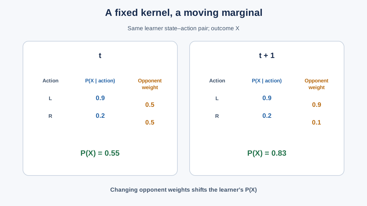
Two agents, two actions each. Agent $i$ chooses $a_i \in \{L, R\}$. The opponent chooses $a_j \in \{L, R\}$. The true transition kernel, for a fixed state $s$ and agent $i$'s action $a_i = L$, is:

$a_j$	$P(s' = X \mid s, L, a_j)$	$P(s' = Y \mid s, L, a_j)$
$L$	0.9	0.1
$R$	0.2	0.8

Now suppose the opponent's policy is $\pi_j(L \mid s) = 0.5$. The effective transition is:

$$P_i(s' = X \mid s, L) = 0.5 \cdot 0.9 + 0.5 \cdot 0.2 = 0.55.$$

The opponent learns. Its policy shifts to $\pi_j(L \mid s) = 0.9$. The same state, the same action $L$, produces:

$$P_i(s' = X \mid s, L) = 0.9 \cdot 0.9 + 0.1 \cdot 0.2 = 0.83.$$

Nothing about the game changed. The kernel is the same table. But the distribution agent $i$ samples from moved from $0.55$ to $0.83$ for an identical $(s, a_i)$ pair. If agent $i$'s value estimate was calibrated to the first number, it is now wrong by a wide margin — and it has no way to tell from the state alone which world it is in.

For agent i choosing L:
Opponent chooses L: P(X) = 0.9
Opponent chooses R: P(X) = 0.2

Stationary, Time-Varying, or Non-Markov?

The slogan "the Markov property fails" is too coarse to be useful, and it hides the distinction that determines which fix you need. Three cases have to be separated.

Case 1: Stationary Markov. The other policies are frozen. $\pi_{-i}$ is a fixed distribution, so $P_i^{\pi_{-i}}$ is a fixed kernel. Agent $i$ faces an ordinary MDP, and single-agent theory applies without modification. This is the regime where treating the environment as an MDP is not sloppy — it is correct.

Case 2: Time-inhomogeneous Markov. The other policies change, but they change as a function of time (or of a training step counter) rather than as a function of the state or history. Then $P_i^{\pi_{-i}^{(t)}}$ depends on $t$, but conditional on $(s, a_i, t)$ the next state is still independent of everything earlier. The process is Markov once you augment the state with time. It is non-stationary, but it is not non-Markov. This is the case the marginalization derivation establishes under its stated assumptions.

Case 3: History-dependent, genuinely non-Markov. The other policies adapt to the history of play — they are themselves learning from the trajectory. Now $\pi_{-i}^{(t)}$ depends on what has happened, and the state-only marginal $P_i(s' \mid s, a_i)$ is no longer a sufficient statistic for the future. The hidden policy state carries information the state does not. This is where the Markov property genuinely fails from agent $i$'s local viewpoint, and where the process becomes partially observable rather than merely time-varying.

The practical consequence is direct. In Case 2, you can restore Markov-ness by conditioning on time or on a training-phase variable. In Case 3, you cannot — you have to condition on the others' behavior, or fold an estimate of it back into the observation. The two cases look identical in a loss curve and demand different remedies.

Common mistake: Treating every policy update as proof that the Markov property broke. A policy schedule that changes over time gives you a time-varying but still Markov process. Reserve the non-Markov claim for when hidden policy state or history affects the conditional transition beyond the current state, action, and time.

What the Formal View Predicts

The derivation is only useful if it makes falsifiable claims about your training runs. It does.

Replay buffers hold stale joint policies. Every transition in the buffer was sampled under some $\pi_{-i}^{(t')}$ with $t' < t$. The empirical distribution in the buffer diverges from the current effective process. Staleness is not a separate bug you can patch; it is a direct consequence of the marginalization. The buffer is a museum of policies that no longer exist.

Drift scales with policy change per update. The size of the shift in $P_i^{\pi_{-i}}$ is bounded by how much $\pi_{-i}$ changes between updates. Slower co-learning and larger batches reduce per-step drift, because they reduce the distance the weights travel per gradient step.

Fixed-kernel convergence guarantees do not apply. The theorems that promise Q-learning converges assume a stationary transition kernel. Your effective kernel is not stationary. This is why you see oscillation and cycling instead of clean convergence — not because your learning rate is wrong, but because the object you are converging toward is being redefined.

A stable-looking policy can be a compromise. A learner can appear to settle on a policy that is actually a weighted average of responses to opponents that have since changed. It looks converged. It is not; it is stranded.

Three diagnostics worth instrumenting:

• Target-value variance across updates. If the TD target's variance is high even with a fixed batch, the target is moving.
• Buffer age distribution. Track how old the transitions in each batch are, in units of opponent updates. A long tail means you are training on ancient policies.
• Frozen-snapshot versus live evaluation. Score your learner against a frozen copy of the other agents, then against the live population. A large gap is the signature of endogenous drift.

Two Kinds of Moving Target

Not every moving target is the same moving target, and conflating them leads to the wrong fix.

Source of drift	What moves	Can one agent cause it?	Class of remedy
Endogenous — other agents' policies	$P_i^{\pi_{-i}}$, $R_i^{\pi_{-i}}$	No; requires other learners	Condition on the joint action, reshape the target, redefine the state
Exogenous — the environment itself	$P$, $R$ directly	Yes; exists even with one agent	Forgetting, windowing, change detection, tracking

Endogenous drift is the subject of this article. It is caused by learning inside the system. Exogenous drift is studied in non-stationary MDP settings and would exist even if you were the only agent in the world.

The distinction matters because the remedies do not transfer. Forgetting old experience helps with exogenous drift — the old data is genuinely from a different world. But forgetting does not fix endogenous drift, because the drift is not in the data's age; it is in the fact that the data was generated under a joint policy that no longer exists. You can have perfectly fresh data and still be chasing a target that moved between collection and update.

In practice both are often present. A measurement that cannot separate them will misattribute the cause, and you will spend a week tuning a forgetting rate for a problem that needed joint-action conditioning.

When the Fixed-Game View Is Still the Right Tool

The theory is not free, and applying it where it does not belong is its own failure mode.

Use the fixed-game view when the other agents are frozen, scripted, or changing on a much slower timescale than your learner. If the opponent updates once per thousand of your updates, the effective process is approximately stationary over your learning window, and standard single-agent reasoning holds.

Use the moving-target view when policies update on comparable timescales, when your own updates feed back into the others' experience, or when evaluation depends on which opponent snapshot you happen to face.

The practical test is a timescale comparison, and it is a heuristic, not a theorem. Measure two things: how often your learner updates, and how much the other policies actually change per update. The second measurement is the one that matters, because update frequency alone says nothing about how far the weights travel. A slow-updating opponent that jumps between near-deterministic policies can move your effective kernel more than a fast-updating opponent that nudges its logits. Anchor the decision in measured policy change — or better, in measured change of the induced kernel $P_i^{\pi_{-i}}$ over your learner's update window. When that change is small relative to the noise in your value estimates, the fixed view is a reasonable approximation and you should not pay the complexity cost of the moving-target machinery. When it is comparable, treat the target as moving.

Common mistake: Assuming that a frozen opponent makes the problem single-agent. It does not — it makes the effective process stationary, which is what single-agent theory actually requires. The distinction is worth keeping straight, because it tells you exactly what you bought by freezing.

Where the theory stops being exact: the marginalization argument assumes the other agents' policies are well-defined distributions at each step. When policies are being updated mid-episode, or when exploration is heavy enough that the "policy" is really a transient, that assumption is a modeling convenience rather than a fact. The derivation still tells you the direction of the drift; it just stops being a precise prediction of its magnitude.

And an honest boundary: this article formalizes the problem. It does not derive a specific algorithm's fix. Do not expect the derivation alone to hand you a stable training recipe — it hands you the term that has to be dealt with, and the choice of how to deal with it is the next article's problem.

Where to Go Next

The tuple is fixed. The induced process is not. The derivation shows exactly which term carries the time dependence: the marginalization over $\pi_{-i}$, and its inheritance of that policy's time index.

The concrete next move is to instrument one training run. Log the buffer age distribution in units of opponent updates. Log the variance of your TD targets across a fixed batch. Then evaluate the same checkpoint twice — once against a frozen snapshot of the other agents, once against the live population. If the two scores diverge, you have measured endogenous drift directly, and you know which regime you are in.

From there, the natural question is how algorithms condition on the joint action or reshape the learning target to restore a stationary objective. That is where the fixes live: centralized critics that take the joint action as input, target networks that lag the moving policy, and state augmentations that fold the others' behavior back into the observation. Each is a different answer to the same equation.