Opponent Modeling in Multi-Agent RL: Predicting the Other Learner

The moment you treat another learning agent as part of the environment, you are betting on a target that moves. Opponent modeling is the attempt to stop guessing and start predicting—but every prediction you add becomes a new assumption that can fail silently.

Why Treating the Opponent as Noise Stops Working

You already know the core problem: when another agent learns, the environment becomes non-stationary from your perspective. Transitions shift, rewards drift, and what worked last episode may be exactly what gets you exploited this one.

The naive response is to fold the opponent into the environment and learn a best response to its average behavior. Marginalize over its actions, treat the other learner as part of the world's dynamics, and run standard single-agent reinforcement learning. If the opponent were stationary, this would be correct—the multi-agent problem would reduce to a single-agent one, and you could ignore the other agent entirely.

But in competitive and mixed-motive settings, the average opponent is a fiction. No single opponent you actually face matches the mean of the distribution you trained against. Best-responding to a fiction leaves you exploitable in two directions: you overfit to behaviors that rarely occur, and you miss systematic patterns that a real opponent repeats every episode.

The core reframe is this: opponent modeling is not about knowing the opponent's true policy. It is about maintaining a live belief—a prediction you update as you observe—and acting on that belief. The question is never "can I read the opponent's mind?" It is "can I maintain a useful estimate of what this particular learner will do next, given what I have seen so far?"

That reframe organizes everything around two questions: what to model, and how to use the prediction.

A Concrete Scenario: The Two-Type Pursuer

Before diving into the taxonomy, let's watch the mechanism move in a minimal setting.

Imagine a repeated pursuit-evasion game. You control an evader. Your opponent is a pursuer with one of two hidden types: Type A commits to the nearest corner before chasing, while Type B immediately chases your current position. Your reward depends on knowing which type you face, because the correct evasive action differs: against Type A you feint toward one corner then break the other way; against Type B you change direction sharply and often.

You observe the pursuer's first two moves. Against Type A, the pursuer's early trajectory bends toward a corner regardless of where you are. Against Type B, its trajectory tracks you directly. Your opponent model takes those observations and outputs a belief: 0.85 that this is Type A, 0.15 that it is Type B. Your policy then conditions on that belief and chooses the feint-and-break maneuver.

Now watch what happens when the model is wrong. If the pursuer is actually Type B but your model is confidently stuck at 0.9 for Type A, you commit to a slow feint. The pursuer closes the distance. Your confident prediction did not degrade gracefully to uncertainty—it actively selected a worse action than a policy that ignored the opponent and simply changed direction often.

This is the entire tradeoff in miniature. The model earns its keep only when its belief shifts your action toward something better than the no-model baseline. And the moment the pursuer learns that you feint against corner-committers, it can fake a corner commitment for two moves, then switch to direct pursuit. Your model, now confidently wrong, drives you into a trap.

Keep this scenario in mind. Every design choice below is really a question about how that belief gets formed, used, and trusted.

What an Opponent Model Actually Predicts

The first design decision is choosing the variable you predict. The choice determines the entire approach, because each target carries different assumptions and different data requirements.

Action prediction is the most direct and least assumption-heavy option. You train a classifier over the opponent's action space, using observed transitions as labels. Given the current state and history, the model outputs a probability distribution over what the opponent will do next. This is behavior cloning applied to the other agent: you watch what it does, and you learn to anticipate it.

Goal or intent inference matters when rewards depend on hidden objectives the opponent reveals only through behavior. In imperfect-information games—poker, negotiation, pursuit-evasion—the opponent's private state drives its actions. You cannot predict its next move well without inferring the hidden goal behind it. The model targets the latent variable, and action prediction falls out as a consequence. In the pursuit scenario, this means inferring the pursuer's type rather than just its next position.

Policy-level models go further. Instead of predicting the next action, they attempt to reconstruct the opponent's policy parameters directly. This is more ambitious: you are not asking "what will it do here?" but "what rule is it following everywhere?"

Learning-dynamics models are the most aggressive target. They try to predict not just what the opponent does now, but how it will change as it learns. This means modeling the opponent's learning algorithm, its update rule, and its trajectory through policy space.

The tradeoff runs along a spectrum: richer targets give more foresight but require more assumptions and more data to estimate reliably. Action prediction needs only observed behavior. Learning-dynamics prediction needs to know something about how the opponent updates—an assumption that is often wrong.

Note: A useful mental image is a spectrum from "predict the next action" to "predict the opponent's learning trajectory." Each step toward the right end buys you more lead time, but each step also demands more evidence and more assumptions about the opponent's internal machinery.

One clarification prevents a common confusion: these are inference targets, not interchangeable model types. Behavior cloning is a training method for action prediction. Self-other modeling—using your own policy to predict the opponent—is a modeling strategy that assumes the opponent reasons like you do. It can serve goal inference or action prediction, but it is not itself a fourth target on the spectrum.

How the Prediction Gets Used

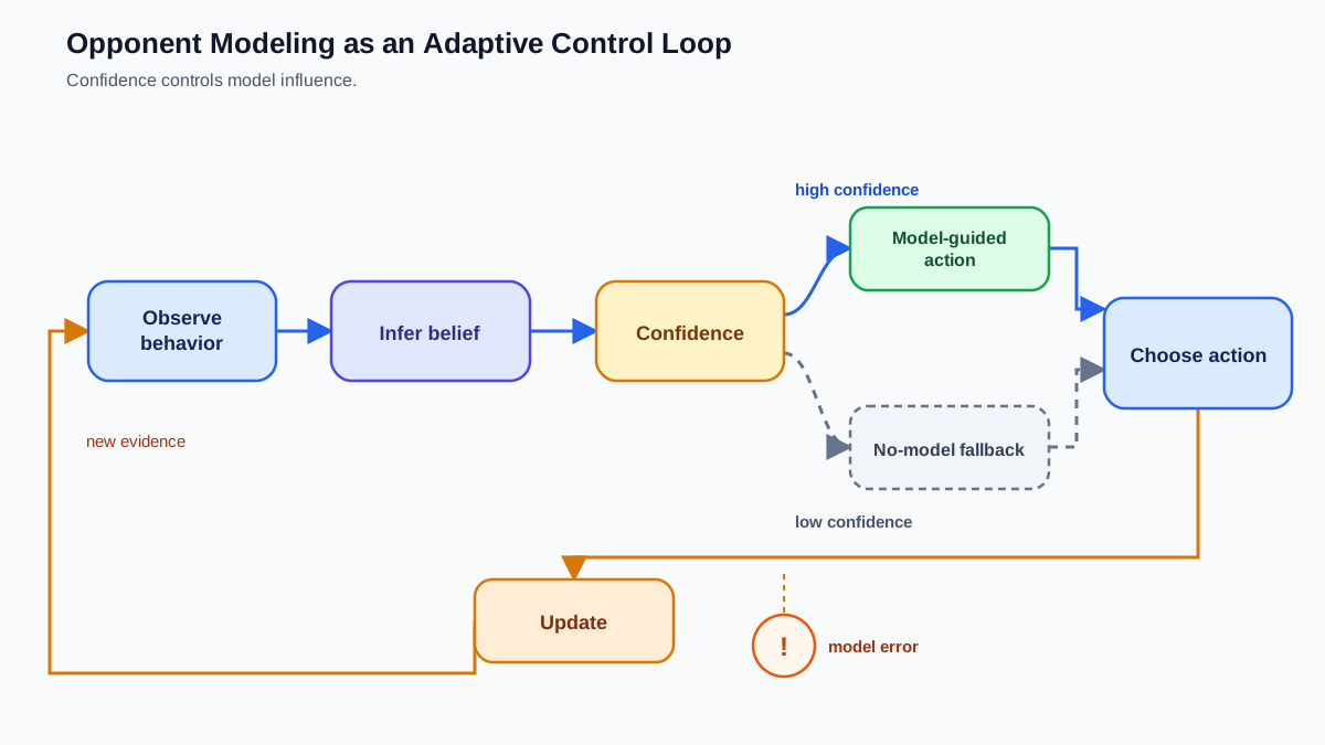
The second design question—how the prediction feeds decision-making—shapes whether modeling helps or hurts more than the accuracy of the model itself.

The most common pattern is conditioning your own policy. The opponent model's output becomes an extra input to your policy network. Your action selection now depends not only on the state but on what you expect the opponent to do. In the pursuit scenario, the belief over pursuer type becomes part of the evader's observation.

A second pattern is feeding a planning or rollout process. Instead of conditioning a policy directly, you use the opponent model to simulate the opponent's likely responses before committing to an action. This matters in settings where you can look ahead: you imagine what the opponent would do in response to each candidate action, and you choose the one that leads to the best outcome under your prediction.

A third pattern is shaping exploration or opponent selection during training. The model steers you toward opponents that expose weaknesses in your current policy, or away from opponents you already handle well. This is less about the current episode and more about the efficiency of the training process itself.

There is an important distinction hiding here: the prediction model and the decision model are separate networks with separate jobs. One estimates the opponent; the other chooses your action. They can be trained jointly or separately, and keeping them conceptually distinct prevents a common failure—treating the opponent model as if it were part of your policy when it is really an input to it.

Why does the use matter more than the accuracy? Because a perfect model you cannot act on is worthless, and a rough model that changes your action distribution can be decisive. A prediction only earns its keep when it alters what you do.

When Prediction Improves Adaptation

Opponent modeling pays off when the opponent's behavior is patterned but not stationary—predictable enough to exploit, changing enough that a fixed best response decays. That combination is the sweet spot. If the opponent were perfectly predictable and never changed, you could learn a static counter-strategy once and stop modeling. If it changed randomly with no pattern, no model could track it. The interesting middle is where behavior carries signal worth extracting.

The technique shines in imperfect-information settings where the opponent's hidden state drives its actions. When you cannot observe the opponent's hand, goal, or resources directly, you must infer them from behavior. In the pursuit scenario, the pursuer's type is unobserved, and the optimal evasive action depends on it. Opponent modeling is not an enhancement in these settings; it is often the only practical way to make good decisions at all.

It also helps when you face a population of heterogeneous opponents rather than one fixed adversary. A single model can adapt per opponent, maintaining separate beliefs for different opponents it encounters. Against a homogeneous population, a static best response may suffice. Against a diverse one, the ability to identify which opponent you are facing and adjust accordingly is what separates robust performance from collapse.

The mental model to install: modeling is a bet that the opponent's behavior carries signal worth extracting. Before building an opponent model, ask whether that bet is likely to pay off in your environment.

When the Model Becomes a Brittle Assumption

The failure modes are where opponent modeling stops being clever and starts being dangerous.

Model error compounds. If the opponent model is wrong, your policy optimizes against a fiction—and can be strictly worse than ignoring the opponent entirely. A bad model does not degrade gracefully to "no model." It actively misleads your action selection toward responses that are wrong for the actual opponent.

The opponent can adapt to your model of it. This creates a second-order loop: your prediction becomes stale the moment it is accurate enough to exploit. You learn to predict the opponent; the opponent learns that you are predicting it and changes; your model, now confidently wrong, drives you into a trap. The target does not just move—it moves because you are tracking it.

Self-other modeling carries a hidden assumption worth naming explicitly. Using your own policy to predict the opponent assumes the opponent reasons like you do. Against a genuinely different learner—one with a different reward structure, a different update rule, or a different level of sophistication—that assumption breaks. You are not modeling the opponent; you are modeling a mirror image and calling it the opponent.

Overfitting to a single opponent during training produces policies that collapse against unseen opponents. The model becomes so tuned to one adversary's quirks that it trades robustness for short-term win rate. This is the classic self-play failure mode reappearing through the opponent model.

Here is the brittle-assumption test: if your model's error is large, or its target moves faster than you can update, the prediction is noise wearing a costume. It looks like information, but acting on it is worse than acting on nothing.

Reading the Tradeoff: Adaptation Versus Model Error

The central tension deserves an explicit frame: opponent modeling trades a bias toward the current opponent for variance from model error. You become more responsive to the specific opponent you face, but you inherit the risk that your estimate of that opponent is wrong. The question is not whether the model is accurate in the abstract. It is whether acting on the model beats acting without it, given the actual error rate.

This is where the evaluation logic needs to be sharper than "track the loss." Predictive fit, calibration, and decision value are three different measurements, and conflating them produces unstable rules.

Predictive fit tells you whether the opponent's behavior is learnable from the data you have. Measure it on held-out trajectories, not just the transitions you trained on. If next-action cross-entropy stays low on held-out data, the opponent is trackable.

Calibration and uncertainty tell you whether the model's confidence matches its accuracy. A model that is right 85% of the time but claims 97% confidence on the states that matter most is dangerous precisely because it will not trigger your fallback behavior. If your policy acts differently under high confidence, you need the confidence to mean something.

Decision value is the only measurement that answers the real question. Remove the opponent model entirely and compare performance against the same population of opponents. If the no-model baseline matches or beats the modeled policy, the model was never doing useful work—regardless of how low its prediction loss looked.

The practical lever is evaluation across a held-out population. Do not measure only win rate against your training opponent. Measure robustness across opponents you never trained against. A model that wins against its training partner but collapses against anything new has not solved the problem; it has memorized a single adversary.

Common mistake: Treating low prediction loss as proof that the model improves control. The most predictable action may be strategically irrelevant. A calibrated but slightly less accurate model can support better planning than a high-accuracy model that is overconfident on important states. Prediction loss is a diagnostic, not the success criterion.

Treat the opponent model like any learned component and debug it the way you would debug a value network that silently fails. Watch its loss on held-out data. Watch what happens to your policy when you ablate the model—remove it entirely and compare performance. If removing the model does not hurt, the model was never earning its complexity.

Decision Boundaries You Can Test

The when-to-use and when-not-to-use rules are not environment labels; they are measurable conditions.

Skip opponent modeling when a no-model baseline matches it. If a fixed best response performs as well against your opponent population, the model is overhead. Test this directly before investing in richer targets.

Skip it when the action space makes prediction statistically hopeless. If you cannot gather enough data to estimate the opponent's behavior, the model will never converge. This is a data-availability test, not a philosophical one.

Add a fallback when identity or data support is weak. If you face a heterogeneous population but cannot reliably identify which opponent you are facing, a per-opponent model can be worse than a robust general policy. Use uncertainty to gate the model's influence: when confidence is low, fall back to the no-model policy rather than acting on a guess.

Keep modeling when hidden state materially affects the optimal action. If the opponent's private information changes what you should do, and you can infer that information from behavior, the model is not a luxury—it is the mechanism that turns observation into advantage.

The durable takeaway: opponent modeling is a tool for turning non-stationarity from a liability into an exploitable signal—but only when you can measure whether the signal is real. Build the model, instrument it, and hold it to the same standard you would hold any other component: does acting on it beat acting without it, across the population of opponents you actually care about?

My rule is simple. Before adding an opponent model, define the test that would convince you to remove it. If you cannot name that test, you are not ready to add the model.

References

Research updated Sep 9, 2026