
Self-Play in Reinforcement Learning: How Agents Learn From Evolving Opponents
The opponent is part of the environment, and the opponent keeps learning. That single fact turns self-play into a moving-target problem where your own…

Key topics
The opponent is part of the environment, and the opponent keeps learning. That single fact turns self-play into a moving-target problem where your own recent output becomes the training signal—and the source of instability.
Why Self-Play Breaks the Single-Agent Assumption
Standard reinforcement learning trains against a fixed environment. Transition dynamics and reward structure stay put while your policy improves. Old experience still describes the same task, and progress can be measured against a stable baseline.
Self-play removes that assumption at the root. When an agent trains against copies or past versions of itself, the opponent's policy is part of the environment. Because the opponent learns too, the transition and reward structure shift under your agent's feet. Every improvement in one agent redefines the task for the other. The same action in the same observed state can produce a different outcome next week because the opponent now responds differently.
This is the non-stationarity problem from multi-agent RL, but self-play gives it a particular shape: the source of instability is not an arbitrary external agent. It is your own learning trajectory reflected back at you. The formal setting is a Markov game rather than a Markov decision process, because the reward depends on the joint action of both players.
Self-play is one way to populate that opponent slot without external data, human demonstrations, or a hand-coded adversary. It generates its own curriculum of challenge. The cost is that the problem your agent is solving keeps changing while it learns. That fact drives every design decision that follows.
Knowledge check
Check your understanding
Answer this question before you continue.
The Self-Play Training Loop
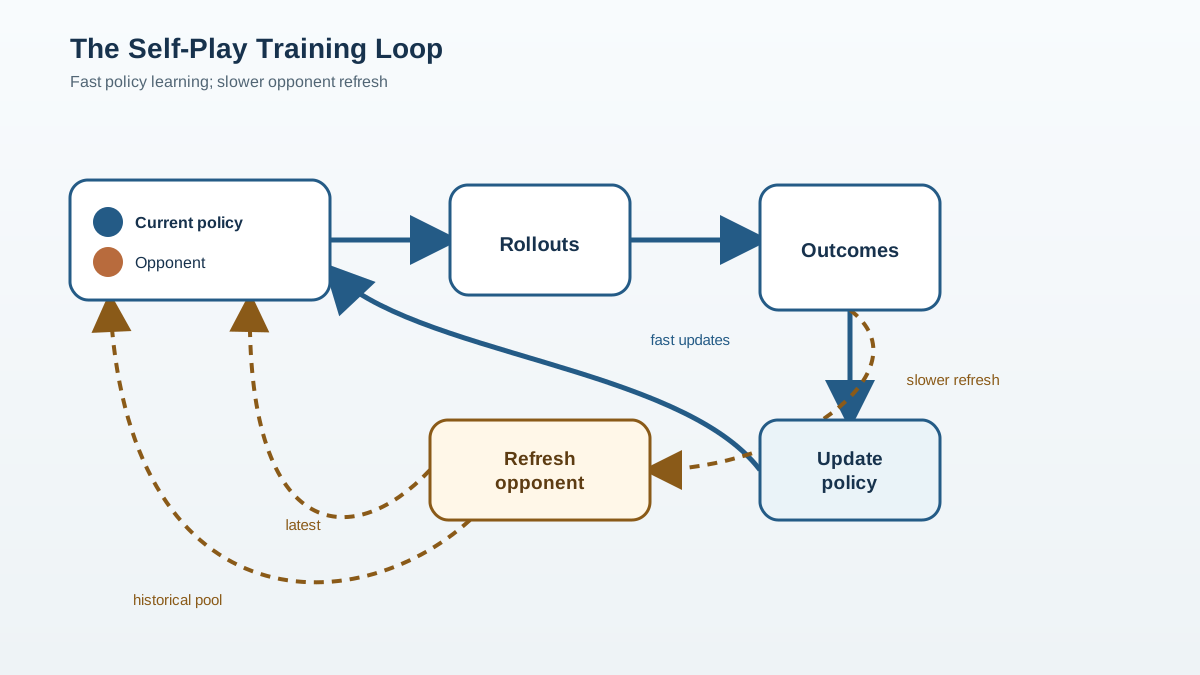
The core loop is simple to state and surprisingly easy to break in practice.
- Instantiate policies. The current policy plays one role; an opponent policy plays the other. In symmetric games, both may be copies of the same model. In asymmetric settings, you may need separate networks for different roles.
- Roll out episodes. The protagonist and adversary interact in the shared environment, generating trajectories.
- Extract the learning signal. Win/loss, reward, or a more nuanced outcome measure becomes feedback for both sides.
- Update the policy. Each agent improves based on what it observed.
- Refresh the opponent. At some interval, decide whether the opponent stays fixed, becomes the latest policy, or is drawn from a pool of historical versions.
A useful mental model: the policy update and the opponent refresh run on separate clocks. The policy updates frequently—every batch or every episode. The opponent refreshes slowly, or according to a selection rule. When those two clocks drift out of sync, the loop breaks in characteristic ways.
A stale opponent means your agent practices against a strategy that no longer represents the real challenge. An overfit-to-self policy means your agent has learned to beat one narrow strategy and nothing else. An update that only wins against the current snapshot means progress is an illusion—the agent has memorized a single opponent's weaknesses rather than generalizing.
Note: In symmetric games, both sides' experience can feed learning because both policies are yours. But the two viewpoints produce correlated trajectories, and whether both are valid training data depends on whether the roles share parameters and how rewards are assigned. Count usable learning signal, not raw episodes.
Knowledge check
Check your understanding
Answer this question before you continue.
Who the Agent Plays Against: Opponent Selection
"Playing against yourself" is not one method. It is a family of choices, and the opponent selection strategy determines almost everything about stability and final performance.
Naive self-play always pits the current policy against the latest version of itself. It is the simplest setup and the most unstable. The opponent chases the current strategy, so the target moves as fast as the learner does. In games with rock-paper-scissors dynamics, the policy can oscillate forever—beating the strategy it just faced and losing to the one before.
Opponent pools preserve historical versions of the policy and sample from them during training. Instead of always facing the latest self, the agent faces a distribution of past selves. This slows the moving target and keeps the policy from specializing against a single recent strategy.
Role-separated designs split agents into main agents and exploiters. Main agents train against the pool using standard self-play. Exploiters are optimized specifically to beat the current main agents, exposing weaknesses that self-play alone would miss. The main agents then train against those exploiters, closing the gaps. This architecture trades simplicity for robustness.
My rule of thumb: naive self-play is cheap and works for symmetric games with small strategy spaces where the equilibrium is easy to reach. Opponent pools and exploiters earn their cost when the strategy space is large, the game is asymmetric, or deployment includes adversaries who will actively search for your weaknesses.
What Opponent Diversity Can and Cannot Do
Diversity is not a nicety. It is the mechanism that prevents overfitting to a single narrow strategy.
An agent that only ever faces its own latest policy can converge to a strategy that beats that one opponent reliably—and loses to anything else. Training win rate looks excellent. Deployment performance is a disaster. The agent has learned a best response to one strategy, not a robust policy for the game.
A diverse opponent set forces the policy to cover a broader region of strategy space. If the agent must beat a pool of historical versions, a current exploiter, and a scripted baseline, it cannot afford to specialize against any single one. It has to find strategies that work across a range of play styles.
But here is the boundary that matters: opponent diversity controls which challenges the agent encounters. It does not control what the agent retains, and it does not prove the agent is robust. Cycling can persist even with multiple opponents when game dynamics reward strategy rotation. Forgetting is an optimization and memory problem—the update that improves performance against the current opponent can overwrite the weights that encoded competence against older ones. And a pool of historical snapshots can be mutually narrow, sharing the same blind spot.
Think of opponent selection as the curriculum, not the certificate. It determines what problems the agent practices. Whether the agent keeps those skills and whether they survive contact with a genuinely strong adversary are separate questions.
Knowledge check
Check your understanding
Answer this question before you continue.
The Three Failure Modes: Cycling, Forgetting, Exploitability
When a self-play run goes wrong, it usually goes wrong in one of three recognizable ways.
Cycling. The policy oscillates between strategies that beat each other in turn, never converging. The mechanism is rock-paper-scissors dynamics: strategy A beats B, B beats C, C beats A, and the learner chases whichever strategy it most recently faced. The symptom is a repeating win-rate pattern against a fixed reference opponent—the agent wins, then loses, then wins again in a cycle that does not decay. Opponent pools break the cycle by preventing the policy from chasing the latest strategy exclusively, though game dynamics can sustain cycling even with a diverse set.
Forgetting. As the policy chases the newest opponent, it loses skills that beat earlier strategies. The mechanism is interference: the policy update that improves performance against the current opponent overwrites the weights that encoded competence against older ones. The symptom is declining performance against a held-out set of past opponents, even as training win rate climbs. Historical sampling keeps past opponents in the training distribution, but retention ultimately depends on how the optimizer balances old and new experience.
Exploitability. The policy has a hidden weakness that a clever adversary can find, even though it beats everything it trained against. The mechanism is a blind spot: no training opponent attacked this particular weakness, so the policy never learned to defend it. The symptom is a large gap between training win rate and performance against an adversarial evaluator—an opponent specifically optimized to beat your policy. Best-response evaluation exposes this gap; exploiters close it during training.
The sharper diagnostic split: opponent selection controls what challenges are encountered, optimization and memory control what is retained, and evaluation tests what survives outside training. A pool addresses the first. It does not guarantee the second, and it cannot certify the third.
Evaluating a Self-Play Agent: The Moving Baseline Problem
Standard single-agent evaluation breaks under self-play for a simple reason: win rate against the current opponent is a moving baseline. A rising curve can mean your agent improved, your opponent regressed, or both. You cannot tell from the curve alone.
The fix is fixed-reference evaluation, but one frozen yardstick is not enough. You need a matrix of references, each answering a different question:
| Reference type | What it tests | Example |
|---|---|---|
| Frozen historical snapshots | Retention: did the agent keep skills it once had? | Past versions of your own policy |
| Scripted or external baselines | Task competence: is the agent good at the game, not just at beating itself? | Hand-coded strategies, human data, or independent agents |
| Adversarial best-response opponents | Exploitability: can a strong adversary find a hidden weakness? | An opponent optimized specifically to beat your current policy |
Frozen snapshots tell you the agent did not forget. Scripted baselines tell you the agent learned something real about the task. Best-response opponents tell you whether a clever adversary can break what the agent learned. Progress against the current self alone tells you nothing.
The evaluation toolkit from single-agent RL—multiple seeds, repeated episodes, learning curves—still applies. But the moving baseline problem is unique to self-play, and it requires fixed references to solve.
Knowledge check
Check your understanding
Answer this question before you continue.
When Self-Play Is the Right Tool
Self-play shines when the hardest opponent you will face is another instance of the same capability class, and when no external data or human demonstrations are available. Games are the canonical case: the best chess player you can find is another strong chess player, and self-play generates an endless supply of them.
Self-play is overkill or wrong in three situations. First, when the task is genuinely single-agent—there is no opponent to model, and a fixed environment already provides the challenge. Second, when a fixed environment already offers a rich curriculum, so the non-stationarity of self-play adds instability without adding signal. Third, when the reward structure is purely cooperative and coordination is the bottleneck—though the boundary is more subtle than "cooperation versus competition."
The real criterion is whether the setup produces useful learning signal. Adversarial self-play is a poor fit when coordination is the bottleneck, because agents optimizing against each other have no incentive to develop joint strategies. But role-based variants can still help in cooperative settings: multiple copies or role-specific policies can generate difficult joint scenarios that a fixed environment never produces. The question is whether the roles share or oppose objectives, and whether the generated interactions stress the skills you actually care about.
The compute and instability costs are real. Self-play multiplies environment interactions—two policies rolling out episodes instead of one—and adds a tuning surface that single-agent RL does not have: opponent refresh rate, pool size, sampling strategy. Every one of those knobs can destabilize training if set wrong.
My decision rule: use self-play when a strong opponent is the scarce resource and you can generate one from your own policy. Skip it when the environment already provides enough challenge, or when the bottleneck is coordination that adversarial competition cannot produce.
The Smallest Experiment That Reveals the Mechanism
The fastest way to make the moving-target mechanism visible is to run a minimal two-player game with naive self-play. Watch the win rate against a fixed reference opponent. If you see cycling—the win rate oscillating instead of climbing—you have seen the moving target in action.
Then add an opponent pool and observe what changes. The cycling should dampen, and the fixed-reference win rate should start climbing instead of oscillating. Then introduce a best-response evaluator and watch for the gap between training performance and adversarial performance.
That sequence forces the core tension of self-play reinforcement learning into the open: the opponent is both the source of challenge and the source of instability. Build the loop, watch it break, and you will understand why every serious self-play system spends as much effort on opponent selection and evaluation as on policy optimization.
Knowledge check
Final check
Finish the article by checking the ideas you just learned.
References
Research updated Sep 9, 2026


