Non-Stationarity in Multi-Agent Reinforcement Learning: Why Yesterday’s Target Moves

Your training curves look beautiful. Reward is climbing, losses are shrinking, and the agent seems to have mastered its task. Then you deploy it against a slightly different opponent, and it collapses. Not a graceful degradation—a full unraveling.

The problem isn't that your agent learned poorly. It's that your agent learned the wrong thing: a policy tuned to opponents that no longer exist. From your agent's perspective, the rules of the game changed because the other players changed their strategies. You weren't aiming at a fixed target. You were aiming at a target that was aiming back.

The Symptom: A Policy That Works in Training and Fails in the Field

In single-agent RL, the environment's transition function is fixed. The only moving part is your own policy. When you train a DQN agent in Atari, the game's dynamics don't change because you got better at them. The rules were written before you arrived, and they stay written.

Multi-agent systems break this assumption. Every agent you train against is also learning, and every update to their policy changes the environment from your perspective. The induced transition distribution—the distribution you're actually trying to approximate—shifts beneath you.

This distinction matters. The physical dynamics of the world—collision physics, goal locations, reward geometry—may be perfectly fixed. What changes is the behavior of the other agents, which conditions how those dynamics unfold for you. A block in a gridworld doesn't move by itself. It moves because another agent learned to relocate it. The underlying rules didn't change; the other player's strategy did.

The core misconception is treating other learning agents as if they were part of a static environment—like furniture in a room that happens to move. But other agents aren't furniture. They're learners with their own objectives, and every gradient step they take rewrites the effective rules of your game.

Randomness vs. Non-Stationarity: Two Different Kinds of Noise

From a single observation, you cannot tell the difference between environmental randomness and another agent's learning. Both look like variance. This is why the misdiagnosis is so common—and so costly.

Environmental randomness is stationary. The transition distribution is fixed, so averaging over enough samples converges to the true expectation. A windy gridworld has a fixed wind pattern. Flip a coin enough times, and the statistics settle.

Other-agent non-stationarity is different. When a peer updates its policy, the distribution your agent samples from changes. The target you're trying to learn moves. No amount of averaging will converge to a target that won't hold still.

Consider two gridworlds. In the first, wind randomly pushes your agent off course—annoying, but the wind's distribution never changes. In the second, another agent is learning to relocate obstacles. Early in training, it moves blocks randomly. Later, it moves them strategically to block your path. The environment hasn't just added noise; it has changed structure, because the other agent's behavior has changed structure.

A time-unaware learner cannot distinguish these cases from its limited observations. Another agent's learning masquerades as environmental stochasticity. The agent tries to explain the aliased signal as randomness, learns a policy that averages over behaviors that aren't randomly distributed, and ends up with something that works against no one in particular.

Why Replayed Experience Goes Stale

Experience replay stabilizes deep Q-learning by decorrelating experience and freezing value targets. In single-agent RL, a stored transition stays valid because the environment dynamics are fixed. The experience you collected yesterday describes a world that still exists today.

Multi-agent RL breaks this contract.

A stored transition encodes the joint behavior of other agents at collection time. When those agents update their policies, your replay buffer fills with ghosts—transitions that describe a world that no longer exists. Training on stale data drifts your value estimates toward an outdated opponent model. The target network, meanwhile, freezes a target that was already wrong before you froze it.

The failure cascade looks like this: your agent samples old experience, learns from it, updates its Q-values toward a policy that peers no longer follow, and then encounters the actual peers, who behave differently than the replay buffer predicted. The mismatch compounds each iteration.

On-policy methods avoid the stale-buffer trap by discarding old experience each iteration. But they feel the moving target more directly. Every policy update is immediately visible in the next batch of rollouts, which means the non-stationarity hits you in real time rather than through corrupted memory. On-policy learning reduces one source of staleness—it doesn't make the environment stationary.

Measuring the Moving Target

You can't fix what you can't measure. But you also can't trust every measurement equally. The probes below are proxies, not direct causal signatures. Each one tells you something useful, and each one has confounders you need to rule out.

Track opponent-policy drift. Log the KL divergence or parameter distance between successive versions of each peer's policy. This measures how much the peer's policy representation is changing. Large divergence between iterations means your peers are updating faster than your agent can track. But parameter distance doesn't always equal behavioral change—a small parameter shift can flip action probabilities, and a large one can leave behavior roughly intact. Pair this with action-distribution comparisons on matched states to confirm that representational drift is behavioral drift.

Monitor value-estimate variance. If Q-value estimates for the same state-action pair swing widely between iterations, learning isn't converging. This is a useful instability signal, but it's not unique to non-stationarity. Function approximation error, bootstrapping, and partial observability can all produce oscillating value estimates with a fixed opponent. Treat Q-swings as evidence of instability, not proof of a moving target.

Compare frozen vs. live evaluation. Train your agent, then evaluate it twice: once against a frozen copy of its peers, once against the live, still-learning versions. A large performance gap between these two evaluations shows that your agent's policy is sensitive to peer-policy version. The frozen evaluation shows what your agent learned against a particular opponent distribution; the live evaluation shows whether that learning still applies as peers continue to adapt.

This is your closest thing to a causal anchor, because it directly controls the variable you suspect. But it measures sensitivity to peer version, not non-stationarity in the abstract. A large gap can also appear if your agent simply learned a narrow policy that only works against one opponent style—which is itself useful information, but not the same diagnosis.

Watch reward-distribution shifts. If reward statistics for a fixed state-action pair change across training epochs, the environment from your agent's perspective is not stationary. This is the most direct measurement available, because it doesn't require you to inspect peer policies at all. The catch: comparing "the same" state-action pair across epochs requires you to actually match states, which is nontrivial under continuous or partial observations. You need a defined evaluation protocol—fixed starting states, matched observation histories, or binned state abstractions—before this comparison means anything.

One discipline note: instrument everything, run many seeds, and remove stochasticity as a confounder before blaming non-stationarity. Deep RL is brittle with respect to random seeds, and ordinary variance can masquerade as a moving target. Run at least three seeds—more if you want to be thorough—before you trust any single diagnosis.

The Freeze Test: Your Diagnostic Anchor

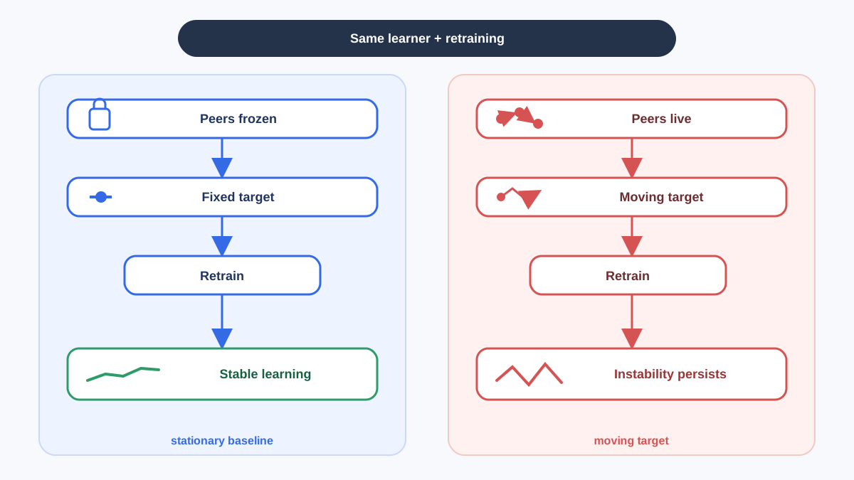
The cleanest experiment for isolating other-agent non-stationarity is the freeze test: freeze all other agents at a fixed policy version and retrain your agent from scratch.

If the instability vanishes against frozen peers, other-agent policy drift is the driver. If it persists, the problem lives elsewhere—in your architecture, your exploration, your credit assignment, or your observation design.

Be precise about what the freeze test proves and what it doesn't. Freezing peers removes peer-policy drift as a variable. It does not prove that your original environment was non-stationary in some absolute sense, and it doesn't distinguish between different sources of peer-induced instability. But it gives you a controlled baseline: a stationary target you can actually hit. If you can't learn against that baseline, you have no business debugging the moving-target case yet.

From there, you can run controlled variations. Retrain against peers that update every N iterations instead of every iteration. Retrain against a population of fixed opponent policies sampled from different training checkpoints. Each variation changes one variable while holding the rest fixed, which is the only way to attribute cause.

When to Suspect Non-Stationarity vs. Other Failure Modes

Non-stationarity is not the answer to every MARL failure. Before you blame the moving target, rule out the other suspects.

Partial observability produces aliasing that looks like noise even with a single fixed opponent. Your agent may be unable to distinguish two world states that require different actions, so its value estimates oscillate as it tries to fit contradictory experience. The diagnostic: give your agent more observation history and see if the instability disappears. If it does, the problem was information, not non-stationarity.

Credit-assignment problems show up as slow or noisy learning even when the environment is stationary. Your agent can't tell which of its actions caused which outcome, so learning crawls. Non-stationarity, by contrast, shows up as divergence or brittleness tied to peer updates.

Deployment mismatch is the case where training was fine but evaluation conditions differ: a different opponent population, a different task distribution, or a different reward scale. This looks like non-stationarity at deployment time, but no amount of training stabilization will fix it if the evaluation distribution was never part of training.

Be honest about the boundary: in practice, these failure modes compound. Partial observability makes non-stationarity harder to detect. Credit-assignment noise obscures the signal of peer updates. The goal isn't to find a single clean cause. It's to isolate the dominant driver so you can pull the right lever.

What the Diagnosis Changes About Your Training Setup

The measurements tell you which lever to pull.

If replay data is stale, the issue isn't buffer age alone—it's the relevance of stored experience to the current behavior policy. A replay buffer that only holds the last few thousand transitions describes a world that approximately still exists. A buffer that holds millions of transitions describes a graveyard of outdated opponent behaviors. If you can, store policy-version metadata with each transition so you can measure how old your data actually is and test whether performance degrades as you include older slices. On-policy methods sidestep this problem by discarding old experience each iteration, but they don't eliminate non-stationarity—they just expose it in real time instead of through corrupted memory.

If the target moves too fast, slow peer updates or stagger learning. Curriculum-style sequencing that limits concurrent policy updates—letting one agent's policy roughly stabilize while another adapts—reduces the moving-target problem by construction. You can't miss a target that isn't moving.

If aliasing is the problem, consider centralized training with decentralized execution. A centralized critic sees the joint state and can condition on other agents' behavior, which reduces the aliasing that makes peers look like noise. This doesn't eliminate non-stationarity, but it gives the learner access to information that makes the environment more legible.

If you're sharing parameters, understand what that changes. Shared networks mean agents co-adapt in lockstep. This can reduce non-stationarity by synchronizing updates, or shift it into a different form, depending on the task. Parameter sharing is a design choice, not a fix.

Each of these is a lever, and the measurement tells you which one to pull. Don't apply all of them at once—you won't know which one worked.

The Diagnostic Workflow

When your MARL training diverges or your policy proves brittle, run this sequence:

1. Freeze all peers and retrain. If the instability vanishes, other-agent policy drift is the driver. If it persists, look elsewhere before blaming non-stationarity.
2. Measure opponent-policy drift. Log KL divergence or parameter distance between successive peer versions, and confirm with action-distribution comparisons on matched states. This tells you how fast peer behavior is actually changing.
3. Monitor value-estimate variance under matched conditions. If Q-values for the same state-action pair swing widely with peers frozen, your instability has a non-stationarity-independent cause.
4. Compare frozen vs. live evaluation. A large gap shows your agent's policy is sensitive to peer version—useful whether the cause is peer drift or narrow overfitting.
5. Pull the lever that matches the measurement. Replay recency for stale experience, update cadence for fast-moving targets, centralized critic for aliasing, broader opponent sampling for narrow policies.

The durable mental model is this: non-stationarity is not noise to average away. It is a target to track. Noise disappears when you collect enough samples. A moving target just keeps moving, no matter how many samples you collect.

Once you can measure the movement, you can decide whether to slow it down, track it more closely, or restructure your learning to see it clearly. That's the difference between diagnosing MARL instability and being confused by it.

References

Research updated Sep 9, 2026