
Stabilizing Deep Q-Learning: Replay, Target Networks, and Moving Targets
Tabular Q-learning converges reliably. Swap the table for a neural network, and the same update can oscillate, blow up, or quietly forget everything it…

Key topics
Tabular Q-learning converges reliably. Swap the table for a neural network, and the same update can oscillate, blow up, or quietly forget everything it learned. The network is not the problem. The target is — or more precisely, the feedback loop between the network, its bootstrapped target, and the data it learns from.
Why the Same Update That Worked in a Table Breaks in a Network
Here is the puzzle worth sitting with: Q-learning has solid convergence guarantees in the tabular case, yet the moment you replace the table with a neural network, those guarantees vanish. The update looks identical. The math feels the same. But something structural changed.
In tabular Q-learning, you update one cell at a time. When you revise the value for state-action pair (s, a), you read the target from other cells in the table — the max Q-value over next-state actions. Those cells do not move during your update. You adjust one entry, the target stays fixed, and the rest of the table waits patiently for its turn.
A neural network does not have cells. It has parameters, and those parameters appear on both sides of the temporal difference error:
TD error = r + γ max Q(s', a'; θ) − Q(s, a; θ)
The predicted value Q(s, a; θ) depends on the weights θ. So does the target r + γ max Q(s', a'; θ). When you take a gradient step and update θ, you do not just move the prediction closer to the target. You move the target itself.
This is the moving-target problem. The network is not chasing a fixed objective the way a table does. It is chasing an objective that shifts every time it takes a step. Imagine trying to hit a dartboard that jumps toward wherever your last dart landed. You can keep throwing, but you cannot tell whether you are improving or just following the board's motion.
This instability is not a minor implementation annoyance. It is the central reason deep Q-learning took years to work in practice, and it is the failure mode that the classic DQN architecture was built to contain.
Knowledge check
Check your understanding
Answer this question before you continue.
The Deadly Triad: Three Ingredients That Turn Learning into Divergence
The moving-target problem does not act alone. Researchers have a name for the full failure recipe: the deadly triad in reinforcement learning. It has three ingredients:
| Ingredient | What it means |
|---|---|
| Function approximation | A neural network (or any parameterized function) generalizes across states instead of storing each one separately |
| Bootstrapping | Updates use a target that includes a current estimate of future value, rather than a complete observed return |
| Off-policy learning | The agent learns from data generated by a different policy than the one being improved |
Each ingredient looks harmless on its own. Function approximation is just generalization. Bootstrapping is what makes temporal-difference learning sample-efficient. Off-policy learning is what lets you reuse experience. But together, they create a feedback loop: the network's own errors feed into the targets, the targets shape the updates, and the updates change the network that produces the next targets. Error does not decay. It amplifies.
The fixes in this article do not remove the deadly triad. DQN still uses function approximation, bootstrapping, and off-policy data. What experience replay and target networks do is dampen the feedback loop — slow it down enough that learning can stay ahead of the instability.
That distinction matters. You are not solving the deadly triad. You are managing it.
Knowledge check
Check your understanding
Answer this question before you continue.
Correlated Experience: Why Consecutive Transitions Lie to the Network
The first failure pressure is the data stream itself. Watch an agent interact with an environment for a few steps, and you will see the problem: consecutive transitions are deeply correlated.
At time t, the agent is in state s_t. It takes action a_t, receives reward r_t, and lands in s_{t+1}. A moment later, it acts again from s_{t+1}. The states are neighbors. The actions were chosen by the same policy. The rewards come from the same region of the environment. If you train on these transitions in order, every mini-batch tells the same story: whatever the agent just did is what the world looks like.
That is a lie by omission. The network overfits to the recent trajectory, forgets older experience, and then the policy shifts in response to what the network learned — which changes the data the agent collects next. The policy and the data chase each other in a loop.
Experience replay breaks that loop. Instead of updating on consecutive transitions as they arrive, the agent stores each transition (s, a, r, s') in a buffer. When it is time to learn, it samples a random mini-batch from the buffer. The samples span many different episodes, many different policies, many different regions of the state space. The temporal correlation is reduced to the point where mini-batches no longer tell a single, misleading story.
Replay has a secondary benefit worth naming: it reuses scarce experience. Every transition can be sampled multiple times, which matters when environment interaction is expensive. But do not mistake the secondary benefit for the primary job. Replay exists first to decorrelate the data stream. Sample efficiency is a bonus.
The practical tradeoff lives in the buffer size. A small buffer holds only recent experience, which means the data still reflects the current policy — correlation creeps back in. A large buffer holds experience from many older policies, which decorrelates better but means the agent learns from increasingly stale behavior. This is why replay only works for off-policy methods: you are explicitly learning from data that an older version of the policy generated.
Common mistake: Treating the replay buffer as a simple memory bank. It is a correlation breaker first and a memory bank second. If your training diverges and your buffer is small, ask whether the data stream became correlated again before you blame the learning rate.
Knowledge check
Check your understanding
Answer this question before you continue.
Moving Targets: Why the Network Chases Its Own Tail
Replay fixes the data stream, but it does not touch the self-referential target. Even with perfectly decorrelated batches, the network still updates toward a target computed by the same weights it is trying to change.
The target network is the remedy for this specific pressure. The idea is almost suspiciously simple: keep a second copy of the Q-network, freeze it, and use only that frozen copy to compute targets. The online network — the one being trained — produces predictions. The target network produces the r + γ max Q(s', a') part of the update. The two networks share an architecture. They do not share a moment-to-moment trajectory.
For a fixed number of steps C, the target network stays frozen. During those steps, the online network chases a genuinely stationary objective. The dartboard stops moving. Then you copy the online weights into the target network, and the cycle repeats.
Classic DQN uses a hard copy: every C steps, the target network's weights are overwritten with the online network's weights. Later methods prefer a soft update: after every step, the target weights move a small fraction toward the online weights, following an exponential moving average. The soft version trades a bit of target staleness for a smoother objective that never jumps.
Here is what the target network does not do: it does not remove the deadly triad. The target still bootstraps. The data is still off-policy. The function approximator still generalizes. What the target network changes is the speed of the feedback. By holding the target fixed for a while, you give the online network time to make progress before the objective shifts again.
Note: The target network and experience replay are complementary, not interchangeable. Replay decorrelates the samples. The target network stabilizes the objective. Remove either one and the other cannot compensate.
Knowledge check
Check your understanding
Answer this question before you continue.
Putting the Two Fixes Together: The DQN Update Loop
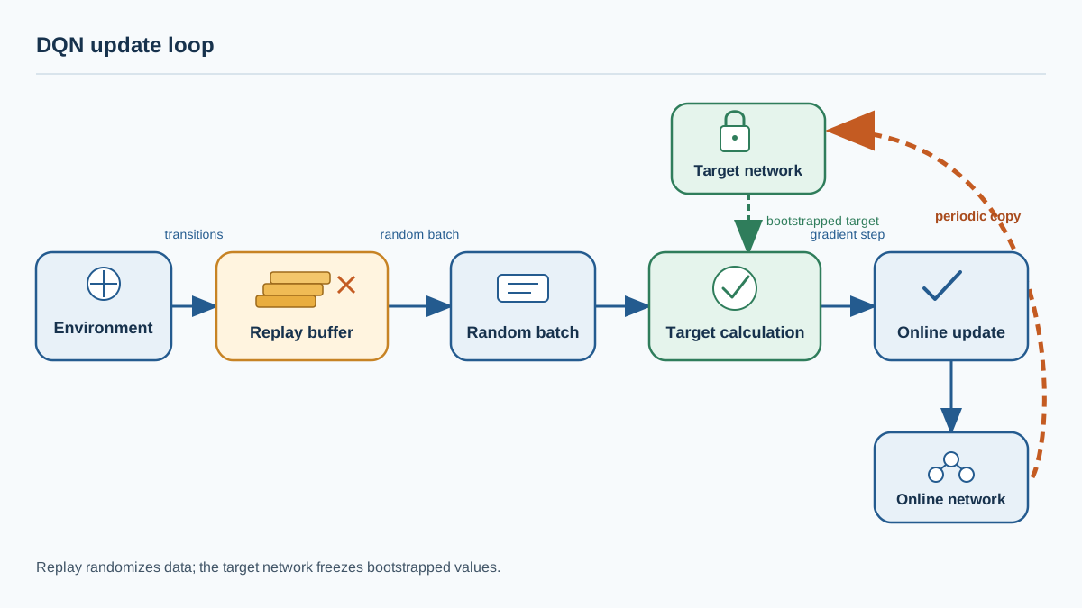
The full DQN update loop shows where each mechanism sits and what it protects against:
- Act. The agent picks an action using an ε-greedy policy derived from the online network's Q-values.
- Store. The resulting transition
(s, a, r, s')goes into the replay buffer. - Sample. When it is time to learn, draw a random mini-batch from the buffer. The randomness is what breaks temporal correlation.
- Compute targets. For each sampled transition, calculate
r + γ max Q(s', a'; θ⁻)using the frozen target network with parametersθ⁻. - Update the online network. Take a gradient step that moves
Q(s, a; θ)toward the target. - Refresh the target. Every
Csteps, copy the online weights into the target network.
┌────────────┐    (s, a, r, s')    ┌────────────────┐
│ Environment│ ──────────────────▶ │ Replay buffer  │
└────────────┘                     └────────────────┘
                                          │
                                          │ random mini-batch
                                          ▼
   ┌────────────────────┐    targets    ┌────────────────────┐
   │ Target network θ⁻  │ ◀──────────── │ Online network θ   │
   └────────────────────┘               └────────────────────┘
           ▲                                      │
           │ periodic copy                        │ gradient update
           └──────────────────────────────────────┘
Two additional stabilizers deserve a mention. Gradient clipping caps the size of each update so a single bad target cannot shove the weights into a destructive region. Reward scaling keeps target magnitudes in a sane range, which matters because the max over actions compounds value estimates and can grow without bound. Neither is as conceptually central as replay or target networks, but both reduce the variance that makes the feedback loop harder to control.
What These Fixes Do Not Solve
Replay and target networks stabilize deep Q-learning. They do not guarantee convergence. The deadly triad can still bite under the right conditions — high discount factors, noisy rewards, or function approximators that generalize too aggressively can all push training back toward divergence.
Two specific failure modes motivated later extensions. Overestimation bias creeps in because the max over next-state actions systematically favors overestimated values; the target network does not remove this bias, it just stops the bias from feeding back instantly. Double DQN addresses it by using the online network to select the best action and the target network to evaluate it. High-variance targets remain a problem when rewards are noisy or the environment is stochastic; later methods address this through distributional value learning and other refinements.
You do not need those extensions yet. What you need is the ability to see the mechanism working — or failing — with your own eyes.
A Diagnostic Experiment: Which Stabilizer Is Doing the Work?
Run a small DQN experiment on a simple environment like CartPole. To make the test meaningful, hold everything else constant: use the same seed, the same network architecture, the same optimizer, the same exploration schedule, and the same number of updates. Change only one stabilizer at a time.
Run 1 — baseline. Train with replay and a target network. Record episode returns, the magnitude of the online network's Q-values, and the spread of TD errors across a fixed evaluation batch.
Run 2 — disable the target network. Keep replay. If the moving-target problem is the dominant pressure, you should see Q-values grow unstable or oscillate even though the data stream is decorrelated. Episode returns may become noisy or diverge. The TD-error spread will widen as the network chases a target that shifts with every update.
Run 3 — disable replay. Keep the target network. If correlated data is the dominant pressure, the network should overfit to its recent trajectory. Episode returns will look good for a stretch, then collapse when the policy shifts and the data distribution changes. The loss curve may actually look fine — which is exactly the trap. Loss can decrease while the policy gets worse, because the network is fitting stale, narrow data.
One run of each is suggestive, not conclusive. Stochastic environments produce noisy curves even with both stabilizers enabled. The diagnostic value comes from comparing the three runs side by side: which failure pattern appears when you remove which mechanism, and does that pattern match the pressure each mechanism was designed to control?
That experiment is the builder's proof. The mental model is not confirmed by reading about the moving-target problem. It is confirmed by watching training diverge when you remove a stabilizer, and by knowing exactly which pressure you let back in.
Knowledge check
Final check
Finish the article by checking the ideas you just learned.
References
Research updated Sep 9, 2026


