
Analyze Cooperation, Competition, and Mixed Motives With Payoff Matrices
Two agents converge. Both policies are stable. Both agents are, by their own local test, optimal. The team still loses.

Key topics
Two agents converge. Both policies are stable. Both agents are, by their own local test, optimal. The team still loses.
That failure is not a training bug. It is a modeling bug, and it comes from a habit we inherit from single-agent RL: treating a policy's quality as a property of that policy alone. In a multi-agent setting, a policy has no intrinsic rank. Its value is defined only relative to what the other players do. Change the opponent, and the ordering of your actions can flip.
The payoff matrix is the smallest tool that makes this explicit. Write down the joint actions, write down what each player gets, and the incentive structure becomes a computable object instead of a debate. A 2×2 grid plus a best-response test tells you whether you are in a cooperative, zero-sum, or mixed-motive regime — and that regime decides what "good" even means.
Why a Single Agent's Return Cannot Rank Policies
A scalar return is only meaningful once the other agents' policies are fixed. Freeze them, and is a well-defined number you can optimize. Unfreeze them, and becomes a function of a moving target.
This is the formal version of the non-stationarity problem. But the payoff matrix gives you a static snapshot you can reason about: hold all other policies fixed, enumerate the joint action profiles, and record what each agent receives. That snapshot is the object you analyze.
A quick bridge from the prerequisite material: the earlier classification of cooperative, competitive, and mixed-motive problems was qualitative. Here we make it computable. The classification stops being a label you assign by intuition and becomes a condition you check on the numbers.
Define the matrix as a map from joint action profiles to per-agent payoffs — not a table of scores. For a two-player game with action sets and , each cell contains a pair .
Convention: the row player's payoff comes first, the column player's second. Every example below follows this. Ambiguity here is the source of most matrix-reading errors.
Knowledge check
Check your understanding
Answer this question before you continue.
Notation and the Three Regimes in One Framework
Fix notation before any derivation.
- Players
- Action sets , with
- Joint profile
- Payoff for player under profile
- Matrix with entries
All three incentive structures are constraints on the same entries.
Cooperative / shared-return. is identical across players, or a monotone transform of a common team return. The matrix has one meaningful number per cell. If the team return is , then with increasing. Maximizing your own payoff and maximizing the team's are the same problem.
Zero-sum. for every profile. The matrix is fully determined by one player's entries. What is good for one is necessarily bad for the other — the sum is constant, so any gain is a transfer.
Mixed-motive / general-sum. The sum varies by cell. Neither alignment nor strict opposition holds. This is the default case, not the exception. Most realistic multi-agent environments blend cooperation and competition, and the matrix makes the blend visible.
Picture one 2×2 grid drawn three times with the same action labels but different payoff entries. The regime is a property of the numbers, not of the game's name. Two environments that look identical in structure can sit in different regimes once you fill in the cells.
Best Response: The Only Local Test That Matters
The best-response operator is the primitive from which every equilibrium claim is built.
Read it carefully: hold the other players' actions fixed at , then choose the action that maximizes your own payoff. The result is a function of the opponent profile, not a constant. "The best action" does not exist in isolation.
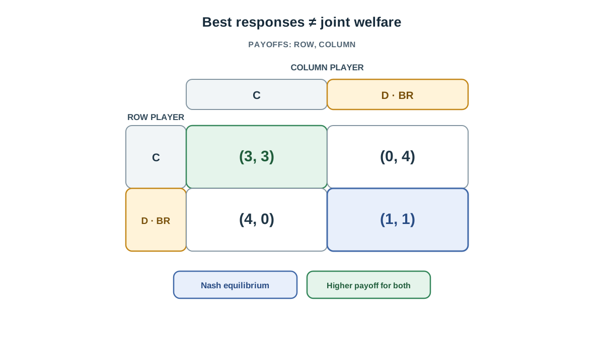
Work a numeric example. Consider this mixed-motive matrix (row payoff first):
| (3, 3) | (0, 4) | |
| (4, 0) | (1, 1) |
Row player's best response, computed column by column:
- Against column : versus . Best response is .
- Against column : versus . Best response is .
The row player's best response is in both columns. That is a dominant strategy — a best response to every opponent profile. Dominance is the special case where the best-response function is constant.
Now the unilateral-deviation test. A profile is stable only if no single player improves by moving alone. Check : row gets 1, and switching to against yields 0. Column gets 1, and switching to against yields 0. Neither improves. is stable.
But note the boundary: best response says nothing about joint welfare. gives a joint payoff of 2. gives 6. Everyone is playing a best response, and everyone is worse off than they could be. That gap is the whole point of the next section.
Knowledge check
Check your understanding
Answer this question before you continue.
Nash Equilibrium and What It Does Not Promise
A profile is a Nash equilibrium when every player's action is a best response to the others' actions in :
Equilibrium is a stability claim about unilateral deviation. It is not a claim about efficiency, fairness, or team performance.
Zero-sum special case. Mutual best response collapses to the minimax value. The value is unique even when the equilibrium policy is mixed. This is the one regime where a single scalar can summarize a policy's quality.
Mixed-motive special case. Multiple equilibria can coexist, and they can differ sharply in joint payoff. The matrix above has one pure equilibrium at , but the profile Pareto-dominates it: both players get 3 instead of 1. The unique equilibrium is Pareto-dominated by a non-equilibrium profile. That is the prisoner's-dilemma shape, and it falls directly out of the entries — no story required.
Common mistake: reading "Nash equilibrium" as "the solution." It is a fixed point of the best-response map, nothing more. A profile can be everyone's best response and still be terrible for everyone.
Knowledge check
Check your understanding
Answer this question before you continue.
Reading a Matrix: A Classification Procedure
Here is a repeatable procedure that turns any small matrix into a regime label plus an equilibrium claim.
Step 1 — Assign the regime. Check whether payoffs are identical (cooperative), strictly opposed with constant sum (zero-sum), or neither (mixed-motive).
Step 2 — Mark best responses. For each player and each opponent profile, mark the cell where that player's payoff is maximized.
Step 3 — Find pure equilibria. Cells where all players' marks coincide are pure-strategy Nash equilibria.
Step 4 — Check for mixed equilibria. If no cell qualifies, look for a mixed equilibrium by equalizing the opponent's expected payoffs across their actions. Solve for the mixing probability that makes the opponent indifferent.
Step 5 — Measure the cooperation gap. Compare the equilibrium joint payoff against the best joint payoff in the matrix. A positive gap means the stable outcome is not the best outcome.
| Regime | Payoff-sum condition | Equilibrium structure | What evaluation should report |
|---|---|---|---|
| Cooperative | Constant across cells | Joint optimum is stable | Team return |
| Zero-sum | Constant (zero) | Minimax value, unique | Exploitability scalar |
| Mixed-motive | Varies by cell | Possibly multiple, possibly mixed | Profile of outcomes across populations |
Knowledge check
Check your understanding
Answer this question before you continue.
How Equilibrium Assumptions Change Policy Evaluation
This is where the formal analysis pays off.
Evaluating against a fixed opponent measures performance in one column of the matrix. It is not a general quality claim. If your opponent happens to play , your policy looks different than if they play .
Evaluating under a best-response opponent measures exploitability — the gap between your current payoff and the payoff you would get against a worst-case responder. In zero-sum settings, exploitability is a well-defined scalar because the opponent's objective is the negative of yours. In general-sum settings, it is not, because the opponent's objective is not the negative of yours. There is no single worst case to measure against.
In mixed-motive settings, report a profile of outcomes across partner and opponent populations rather than a single number. The matrix tells you which populations matter: the columns are the opponent profiles you need to cover.
Warning: reporting a self-play score as if it were an equilibrium value silently assumes the other agents are frozen at their current policies. That assumption is exactly what multi-agent learning violates.
When the Matrix View Stops Being Enough
The static matrix is a lens, not a complete model. Know where it breaks.
A payoff matrix describes a single simultaneous interaction. Repeated interaction, reputation, and punishment are outside it. Sequential and imperfect-information games need the extensive form, not a single grid. Continuous or large action spaces make explicit enumeration impossible, so the matrix becomes a local approximation around a profile.
The sharpest limit: learned policies move the entries. The matrix is only stationary if the other agents' policies are held fixed — which is precisely what multi-agent learning violates. Use the matrix to reason about incentives and evaluation targets, not to predict the trajectory of a learning run.
The Decision Rule
Before scoring any multi-agent policy, write down the matrix. Name the regime. State which opponent profile the score assumes.
That three-step discipline catches the most expensive evaluation error in multi-agent work: a number that looks like a quality claim but is really a measurement against one frozen opponent.
The next practical step is to build a small best-response evaluator for a 2×2 environment. Compute the exploitability gap, then change the opponent's policy and watch the gap move. When you see the number shift under your feet, the payoff-matrix view stops being notation and becomes a tool you reach for before every evaluation.
Knowledge check
Final check
Finish the article by checking the ideas you just learned.
References
Build a stronger RL mental model
Use structured resources to connect equations, algorithms, and observable agent behavior.


