Test Self-Play for Cycling and Exploitability in a Small Game

A self-play win rate can climb for a thousand iterations and still be lying to you. Here is the smallest instrument that catches it.

Self-play reward measures your policy against a target that is running away at the same speed. When both agents improve together, the score rises. When both agents drift into a weak but stable convention, the score also rises. When the pair locks into a rotating cycle of best responses, the score stays flat while the policies underneath it spin. The number cannot tell these apart, because it was never designed to.

This tutorial builds a minimal experiment that can. You will implement self-play in a repeated two-action game, log the full policy vector at every iteration, and evaluate checkpoints against a frozen panel of diverse opponents. By the end you should be able to produce two artifacts from your own run: a policy-history trace that makes cycling visible, and an opponent matrix that exposes exploitability the self-play curve hides.

The self-play loop itself and the general case for diverse evaluation are assumed background here. We are going straight to the measurement.

Why a Self-Play Score Is Not a Progress Bar

Three failure signatures matter, and they look identical in a reward plot.

Cycling is when policies rotate through a repeating sequence of best responses. Agent A shifts toward action 1, so B shifts toward action 2, so A shifts back, and the pair orbits a fixed point instead of settling on it. Exploitability is when a policy is strong against its training partner and weak against an opponent it never saw. The self-play score stays high because the partner is the only thing it was ever measured against.

Both failures share a root cause: non-transitivity. In many games, A beats B, B beats C, and C beats A. When that is true, no single scalar can rank policies, and no single opponent can certify one. A score is a projection of a high-dimensional trajectory onto one number, and the information you need lives in the dimensions that projection throws away.

That is the whole argument for the rest of this article. If you want to see learning, you have to record the policy, not just its payoff.

Choosing a Game Small Enough to Inspect

I want a game whose entire policy fits on one screen. Four requirements:

• A small discrete action set.
• A small state or history space.
• A zero-sum or near-zero-sum payoff.
• A payoff structure that rewards mixing rather than a single dominant action.

A repeated two-action game with a non-transitive payoff matrix satisfies all four. The key property is that no pure action is safe: if you always play action 0, a competent opponent punishes you, and the same is true for action 1. That is what forces the policy to keep moving instead of parking on a dominant action.

Warning: If your payoff matrix has a pure dominant strategy, self-play will converge trivially and the experiment is dead on arrival. Check the matrix before you write the loop. If one action dominates regardless of the opponent, you have built a game that cannot cycle, and you will learn nothing about cycling.

The payoff matrix is the only place the game's difficulty lives. Everything else in this tutorial is instrumentation.

One boundary worth stating plainly: results from a two-action game do not transfer to deep multi-agent settings. The measurement discipline does.

Setting Up the Minimal Self-Play Loop

Dependencies: Python 3 and NumPy. No deep learning framework, no external services, no credentials. You can run this immediately.

Represent the policy as a table of action probabilities per state. In a two-action game with no state beyond "it is my turn," that is a single probability vector of length two, and you can print it, diff it, and plot it.

import numpy as np

# Row player payoff matrix. Row action i, column action j.
# Non-transitive: no pure action dominates.
PAYOFF = np.array([
    [ 1.0, -1.0],
    [-1.0,  1.0],
])

def sample_action(probs, rng):
    return int(rng.random() < probs[0])

def play_episode(row_policy, col_policy, rng):
    a = sample_action(row_policy, rng)
    b = sample_action(col_policy, rng)
    return PAYOFF[a, b]

def update(policy, action, reward, lr=0.05):
    # Simple policy-gradient step on a two-action simplex.
    grad = np.zeros(2)
    grad[action] = reward * (1.0 - policy[action])
    grad[1 - action] = -reward * policy[1 - action]
    policy = policy + lr * grad
    policy = np.clip(policy, 1e-3, 1.0)
    return policy / policy.sum()

The self-play loop samples both roles from the current policy, plays an episode, computes the reward, and updates:

rng = np.random.default_rng(0)
policy = np.array([0.5, 0.5])
history = []

for step in range(2000):
    history.append(policy.copy())
    a = sample_action(policy, rng)
    b = sample_action(policy, rng)
    reward = PAYOFF[a, b]
    policy = update(policy, a, reward)

Print policy every hundred iterations. You should see the numbers move before you plot anything. That is the point: the update rule matters far less than what you record. Swap in regret matching or a tabular Q-learner if you prefer; the experiment's value comes from the logging, not the learner.

Logging Policy History So Cycling Becomes Visible

Record the full policy vector at every iteration. Reward is a scalar projection of a high-dimensional trajectory, and it loses exactly the information you need to distinguish convergence from cycling.

Plot action probabilities over iterations. A converging policy flattens toward a fixed point. A cycling policy traces a closed loop or a slow rotation. Those two shapes are visually distinct, and neither is visible in the reward curve.

Add a short cycle detector:

def find_cycle(history, tol=0.02):
    n = len(history)
    for lag in range(2, n // 2):
        if np.allclose(history[-1], history[-1 - lag], atol=tol):
            return lag
    return None

Do not build a general-purpose detector. A near-repeat check against policies from k iterations ago is enough to flag the pattern for a human to inspect.

Common mistake: A policy can appear to converge while actually oscillating with a period longer than your logging window. Log more iterations than you think you need. If your run is 2000 steps and your cycle period is 3000, you will see a flat line and conclude the wrong thing.

The interpretation rule is simple: if the policy vector returns to a previous value while reward stays flat, you are watching cycling, not learning.

Building a Fixed Diverse Opponent Panel

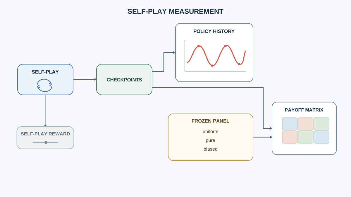
This is the core measurement contribution. Freeze a panel of opponents before training starts:

• A uniform-random policy.
• A pure-action policy for each action.
• One or two fixed mixed policies with different biases, for example [0.8, 0.2] and [0.2, 0.8].

Freeze means freeze. These policies must not update during training. If they move, the panel becomes another moving target and reproduces the original problem.

Evaluate the trained policy against every panel member at regular checkpoints and store the results as a matrix of checkpoints by opponents:

PANEL = {
    "uniform":  np.array([0.5, 0.5]),
    "pure_0":   np.array([1.0, 0.0]),
    "pure_1":   np.array([0.0, 1.0]),
    "biased_a": np.array([0.8, 0.2]),
    "biased_b": np.array([0.2, 0.8]),
}

def evaluate(policy, opponent, episodes=500, rng=None):
    rng = rng or np.random.default_rng(1)
    total = 0.0
    for _ in range(episodes):
        a = sample_action(policy, rng)
        b = sample_action(opponent, rng)
        total += PAYOFF[a, b]
    return total / episodes

Diversity in the panel matters more than strength. A panel of strong-but-similar opponents will miss the same weaknesses a single opponent misses. You want opponents that disagree with each other about what a good policy looks like.

Expected output: a small table of expected payoffs, one row per checkpoint, one column per opponent. You can read it directly.

Reading the Opponent Matrix: Exploitability and Non-Transitivity

Two signatures to look for.

Exploitability shows up as a gap. High payoff against the self-play partner, near-zero or negative payoff against a specific panel member. That gap is the exploit. The policy found something that beats its training partner and nothing else.

Non-transitivity shows up as an inconsistent ordering. Your policy beats opponent A, loses to B, and B loses to A. No consistent ranking exists, so no single ranking is meaningful.

Put the self-play reward curve next to the panel results. The divergence between them is the finding. Show it, do not assert it.

Note: The matrix bounds performance against the panel, not against all policies. A clean panel result is evidence of robustness, not proof of it. Treat it as a lower bound on exploitability, not a certificate of safety.

The decision rule: if panel performance tracks self-play performance, the training signal is informative. If it diverges, trust the panel.

When Self-Play Cycling Is a Bug and When It Is the Game

Cycling is expected when the game has no pure-strategy equilibrium and the learner is deterministic or near-deterministic. The fix is more mixing, not more training. A policy that keeps moving may be closer to correct than one that freezes.

Cycling is a bug when the game has a stable equilibrium and the learner oscillates because of an oversized update step or a stale opponent snapshot. The fix is a smaller step or a slower opponent refresh.

The practical diagnostic: shrink the learning rate and watch the cycle period. If the period shrinks with it, you are looking at an optimization artifact. If it does not, the cycle is structural.

Warning: Damping the learning rate to kill a structural cycle produces a policy that is stable and exploitable. You will have traded a visible problem for an invisible one. Check the panel matrix before you celebrate the flat line.

One Modification Worth Running Next

Replace current-opponent self-play with a snapshot opponent: train against a frozen copy of the policy from N iterations ago, refreshed periodically.

Predict the outcome before you run it. Snapshot opponents should reduce cycle frequency but may slow adaptation and increase exploitability against the panel. If your prediction is wrong, you have learned something about which mechanism was driving the cycle.

Compare the two runs on the same panel matrix. The comparison isolates whether the cycling came from the opponent's co-adaptation or from the learner itself. Keep the change small enough that you can attribute the difference to one variable.

What to Carry Forward

Never trust a self-play curve as a progress signal. Always keep a frozen diverse opponent panel. Always log the policy vector, not just the reward.

The panel is the instrument. The self-play score is only the training signal. That distinction scales all the way up: in larger multi-agent settings, the same discipline applies, and the same failure modes hide behind the same smooth curves.

Run the snapshot-opponent variant. Compare the two panel matrices. The gap between them is where the real lesson lives.