
Exploitability in Multi-Agent Reinforcement Learning: Best Responses and a Worked Game
A policy that wins 90% of its self-play games can still lose to an opponent that never appeared in training.

Key topics
A policy that wins 90% of its self-play games can still lose to an opponent that never appeared in training.
That sentence is the whole reason this metric exists. Self-play score tells you how your policy performed against the opponents it actually met. Exploitability tells you how much a single opponent could gain by choosing the worst possible response to your policy — whether or not that opponent was ever in your training population. Those are different questions, and only one of them is a worst-case bound under a stated model.
This tutorial turns the vague worry into one number, computed by hand on one small game, with every assumption stated out loud.
Why Self-Play Score Is Not a Safety Certificate
You already know the self-play loop: agents train against copies or snapshots of themselves, the opponent distribution shifts as training progresses, and the win rate against that moving population becomes your progress signal. That loop is genuinely useful. It generates opponents of increasing difficulty without you having to hand-author them.
But read what the number actually measures. A self-play win rate is a sample from one distribution of opponents — the ones your training process happened to produce. It says nothing about opponents outside that distribution. A policy can dominate its sparring partners and still leave a wide, cheap-to-find hole for a different opponent.
The hidden question behind "is my policy good?" is usually this: how much can a single opponent gain by deviating to their best response? That is the question exploitability answers, and it is a worst-case question, not an average-case one.
The Setting: Two-Player Zero-Sum, and Why It Must Be Stated First
Exploitability is not a universal score. It is a property of a game plus a policy profile. Change the game and the number changes. So state the assumptions before writing any formula.
This tutorial defines the common two-player zero-sum version. In general-sum games you can still define player-wise deviation gains — each player's best response against the others is well-defined — but those gains do not collapse into the single clean scalar below, and they do not inherit the same equilibrium interpretation. The zero-sum structure is what makes the number mean what people assume it means.
We work with a two-player zero-sum normal-form game:
- Two players, one payoff matrix , where is the payoff to player 1 when player 1 plays action and player 2 plays action .
- Zero-sum: player 2's payoff is exactly . Player 1's gain is player 2's loss, so a single matrix describes the entire game.
- Mixed strategies: a policy is a probability distribution over actions, not a single action. A deterministic policy is exploitable whenever the chosen action has a profitable counter-action — if your opponent knows your one action and a punishing response exists, they take it. Mixed strategies matter precisely when your best response depends on the opponent's predictable choice.
Write for player 1's mixed strategy (a distribution over rows) and for player 2's (a distribution over columns). The expected payoff to player 1 under the profile is
Everything below is built from this one object. Player 2's expected payoff is by the zero-sum assumption.
Note: The zero-sum structure is doing real work. It guarantees that a single value describes the game, which is what lets us define a clean best-response gap. Outside this setting, deviation gains still exist, but they need a different interpretation and do not reduce to this scalar.
Knowledge check
Check your understanding
Answer this question before you continue.
Best Response: The Adversary You Should Assume Exists
Fix player 1's strategy . Player 2 now faces a simple problem: choose to maximize their own expected payoff, which means minimizing .
Because is linear in , the maximum over distributions is attained at a single action. There is no benefit to mixing when you already know the opponent's strategy. So the best response reduces to picking the best column:
Read that carefully. For each column , compute the expected payoff of that column against . Then take the minimum — the column that hurts player 1 the most. That minimum is the value player 2 can guarantee against this specific .
By symmetry, player 1's best response against a fixed is
The best response is not a smart opponent. It is the most inconvenient one. It is allowed to know your strategy and pick the worst column for you. That is the adversary you should assume exists when you claim a policy is strong.
Knowledge check
Check your understanding
Answer this question before you continue.
Defining Exploitability as a Best-Response Gap
Now assemble the definition. The best-response gap for a player is the difference between what they could get by deviating and what they actually get under the current profile.
For player 1, playing against :
For player 2, the same idea from their side. Since player 2's payoff is , their gain from deviating is
Exploitability combines both one-sided gaps. The common form is the average:
A profile with zero exploitability is a Nash equilibrium in this setting: neither player can improve by deviating. Small exploitability means approximately so.
Two things to keep straight:
- Each gap is one-sided. Player 1 is measured against the best they could have done, not against player 2's actual play. The two gaps are computed independently.
- Normalization is a choice. Some report the sum, some the average, some a per-player maximum. Reported exploitability numbers are only comparable when the normalization matches. When you read a number, find out which convention produced it.
Knowledge check
Check your understanding
Answer this question before you continue.
A Worked Game: Computing the Gap by Hand
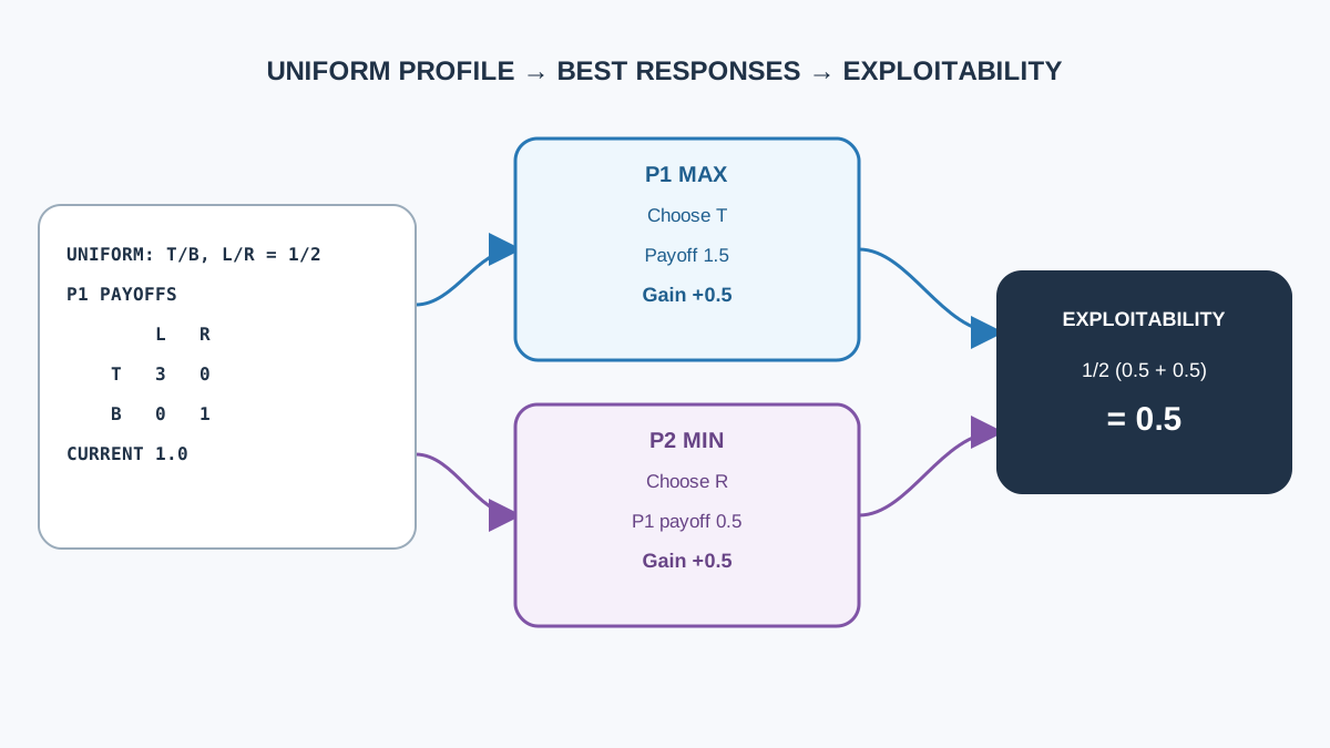
Let's carry one matrix end to end. Consider this 2×2 zero-sum game, with payoffs to player 1:
| 3 | 0 | |
| 0 | 1 |
Start with a deliberately non-equilibrium profile. Suppose both players are playing uniformly:
Step 1 — current payoff. Compute :
Step 2 — player 1's best response. For each row, compute the expected payoff against :
- Row : .
- Row : .
The maximum is , so , and
Step 3 — player 2's best response. For each column, compute the expected payoff to player 1 against :
- Column : .
- Column : .
Player 2 minimizes player 1's payoff, so , and
Step 4 — exploitability.
Interpretation: against this uniform profile, each player can gain in expected payoff by switching to their best response. The profile is far from equilibrium.
Step 5 — sanity check at equilibrium. The equilibrium here is for player 1 to play with probability and with probability , and player 2 to play with probability and with probability . Plug these in:
- .
- Row against : . Row : . Both rows tie at , so and .
- Column against : . Column : . Both tie, so and .
The gap collapses to zero. That is the definition doing exactly what it claims: at equilibrium, no unilateral deviation helps.
Knowledge check
Check your understanding
Answer this question before you continue.
What Exploitability Does Not Measure
This is where the metric gets misused, so draw the boundary sharply.
| Concept | What it measures | Where it applies |
|---|---|---|
| Exploitability (this formulation) | Worst-case gain from a unilateral best response, combined into one scalar | Two-player zero-sum |
| Player-wise deviation gain | One player's best-response improvement | Any game, with a different interpretation |
| Self-play score | Average performance against a training population | Any game with a defined opponent set |
| Robustness across partners | Performance with varied teammates | Cooperative or mixed-motive settings |
- It is not robustness across partners. In a cooperative or mixed-motive game there is no single adversary whose gain is your loss, so the zero-sum scalar does not transfer. Player-wise deviation gains can still be computed, but they answer a different question and do not carry the same equilibrium meaning.
- It is not a general skill score. A low-exploitability policy can be conservative and weak against non-adversarial opponents. Minimizing worst-case loss is not the same as maximizing average reward.
- It is not cleanly defined beyond two players. The equilibrium guarantees that make the metric meaningful weaken in general-sum and many-player games. Counterfactual regret minimization, for instance, provably converges to a Nash equilibrium in two-player zero-sum games but not necessarily with more than two players.
- It is not a training signal by default. It is an evaluation quantity. Computing it requires solving a best-response problem, which is itself expensive in large games.
When to Reach for Exploitability — and When Not To
My rule is simple: reach for exploitability when the game is genuinely two-player zero-sum and you need a worst-case bound rather than an average-case score. That is the setting where the number means what people assume it means.
Do not use it as the headline metric for cooperative teams, mixed-motive settings, or population-based training where partner diversity is the real question. In those settings, exploitability answers a question nobody asked.
A practical cost note: exact best responses are tractable in small games like the one above. In large games, the number becomes an approximation, and you should report it as one. An exact exploitability value in the stated game bounds unilateral improvement under that model; an approximate best response gives an estimate or bound only to the extent its error is controlled. Pair it with population-based evaluation rather than replacing it — the two answer different questions. Population testing asks "how do I do across the opponents I might meet?" Exploitability asks "how much can one adversary take from me?"
The Habit to Build
Before you quote a self-play win rate as evidence of policy quality, ask three questions. Is the game two-player zero-sum? Is a best response computable? What is the gap?
If the answer to the first is no, exploitability is the wrong tool and you should say so. If it is yes, compute the number.
Your next step: take your own small game or toy matrix and compute the best-response gap by hand, exactly as we did above. Then compare it against the self-play score you were already tracking. Where the two disagree, you have found the hole your training population never showed you.
Knowledge check
Final check
Finish the article by checking the ideas you just learned.
References
Build a stronger RL mental model
Use structured resources to connect equations, algorithms, and observable agent behavior.


