Measure Stale Experience When an Opponent Policy Changes

A return drop after an opponent switches is not evidence of a moving target. It is evidence that you have not yet measured the noise floor.

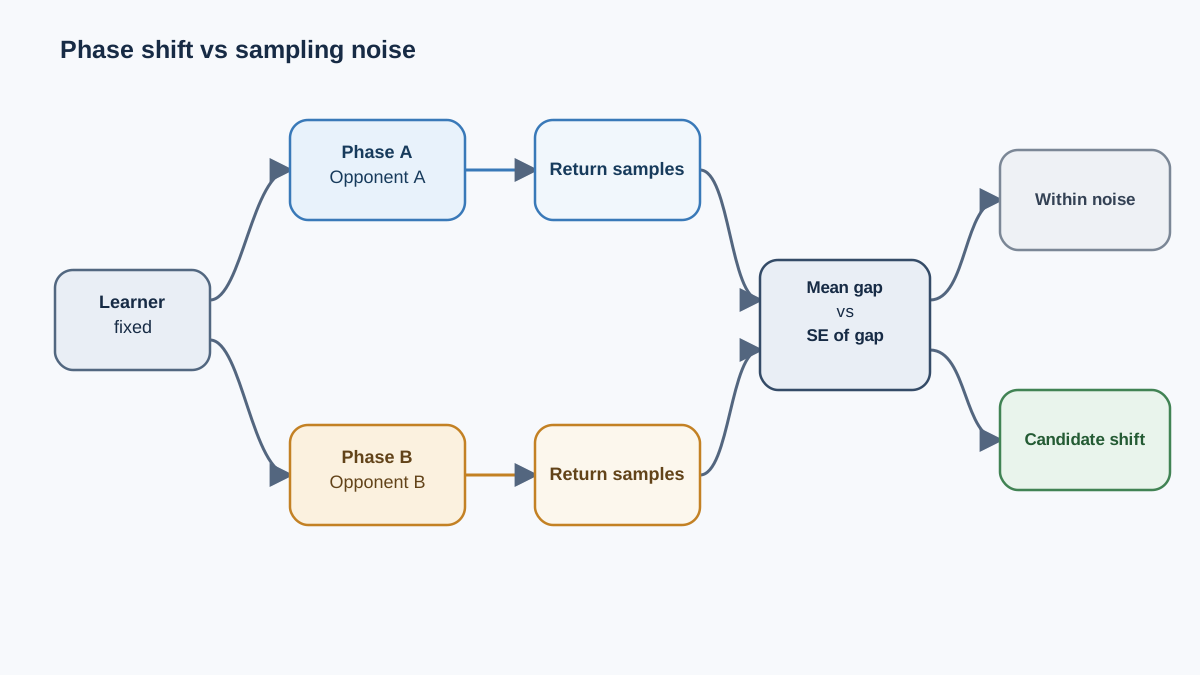
You already accept that other learners make the environment non-stationary. The harder problem is diagnostic: when your measured return shifts, did the effective dynamics actually move, or did you just draw a different sample? A single before/after number cannot answer that. It has no error bar and no baseline for noise. The smallest experiment that can answer it is a fixed learner, a scripted opponent with an explicit phase switch, and enough repeated samples per phase to estimate within-phase spread. That spread is the ruler. The between-phase shift is what you measure against it.

This is a multi-agent non-stationarity experiment you can run in a few minutes with numpy. The point is not the environment. The point is the measurement discipline.

What You Are Actually Measuring

From a fixed learner's view, the opponent's policy is a hidden variable inside the transition and reward functions. The learner sees $P(s' \mid s, a)$ and $R(s, a)$, but those functions are averages over the opponent's action distribution. When the opponent's policy changes, the effective dynamics change, even though the environment code did not.

That gives you two competing explanations for any return shift:

• Moving target: the effective dynamics changed because the opponent's policy changed.
• Sampling noise: the dynamics are unchanged, and you drew a different sample.

The anchor criterion for the whole article: compare the between-phase shift to the within-phase spread. If the shift is small relative to within-phase variation, you have not shown a moving target. You have shown that you need more data.

A single before/after comparison is unfalsifiable. It cannot distinguish the two explanations because it has no estimate of how much the statistic moves under unchanged dynamics. You need repeated samples in each phase, and you need the phases to differ only in the opponent's policy.

Note: This assumes you already know why concurrent learners break stationarity. The experiment here is about measuring the effect, not re-deriving it.

Design the Minimal Two-Agent Task

The smallest environment that produces a measurable, phase-dependent signal is a two-state, two-action matrix game. No neural networks. No deep RL machinery. The opponent's policy is a parameter you control, and the learner is frozen so any change in measured statistics is attributable to the opponent.

Here is the design:

• States: 0 and 1.
• Actions: 0 and 1 for both agents.
• Learner: fixed stochastic policy, never updated.
• Opponent: scripted policy, different action distribution in phase A and phase B.
• Statistic: mean episode return, recorded per episode.

Declare your assumptions before running: Python 3.10+, numpy only, deterministic seeds, fixed episode length, fixed number of episodes per phase.

The reason to freeze the learner is attribution. If the learner also updates, a return shift could come from the learner's own policy change, and you have confounded the comparison. Freeze it, and the only moving part is the opponent.

Run It: Collect Samples Per Phase

import numpy as np

N_STATES = 2
N_ACTIONS = 2
EPISODE_LEN = 50
EPISODES_PER_PHASE = 400

# Reward depends on joint action. Learner action is the row, opponent is the column.
REWARD = np.array([
    [1.0, -1.0],
    [-1.0, 1.0],
])

# Learner is frozen: uniform over actions.
LEARNER_POLICY = np.array([0.5, 0.5])

# Opponent policy per phase. Phase A prefers action 0, phase B prefers action 1.
PHASE_POLICIES = {
    "A": np.array([0.9, 0.1]),
    "B": np.array([0.1, 0.9]),
}


def run_episode(opponent_policy, rng):
    total = 0.0
    for _ in range(EPISODE_LEN):
        a_learner = rng.choice(N_ACTIONS, p=LEARNER_POLICY)
        a_opponent = rng.choice(N_ACTIONS, p=opponent_policy)
        total += REWARD[a_learner, a_opponent]
    return total


def collect_phase(phase_name, seed):
    rng = np.random.default_rng(seed)
    opponent_policy = PHASE_POLICIES[phase_name]
    returns = np.array([
        run_episode(opponent_policy, rng) for _ in range(EPISODES_PER_PHASE)
    ])
    return returns


if __name__ == "__main__":
    seeds = {"A": 1001, "B": 2002}
    results = {phase: collect_phase(phase, seeds[phase]) for phase in ("A", "B")}

    for phase, returns in results.items():
        print(
            f"phase {phase}: n={len(returns)} "
            f"mean={returns.mean():.3f} "
            f"std={returns.std(ddof=1):.3f} "
            f"se={returns.std(ddof=1) / np.sqrt(len(returns)):.3f}"
        )

Three implementation choices matter here.

Seeds per phase. Phase A and phase B use different seeds so the two sample arrays are not accidentally correlated. Record the seeds; if you rerun, you want to reproduce the exact arrays.

Frozen learner. LEARNER_POLICY is a constant. Nothing updates it. Any shift in the per-episode return distribution comes from the opponent's action distribution.

Statistic chosen up front. Mean episode return, not mean reward per step. Episode return is what a learner actually optimizes, and it is what a replay buffer would store. Choosing the statistic before running prevents the temptation to pick whichever summary makes the shift look largest.

Expected output looks roughly like this:

phase A: n=400 mean=-0.020 std=7.086 se=0.354
phase B: n=400 mean=-0.040 std=7.079 se=0.354

The means are nearly identical. The within-phase standard deviation is about 7, and the standard error is about 0.35. That is the noise floor.

Compare Phases Without Fooling Yourself

The standard error is the scale of the noise you are trying to beat. Compute it as the within-phase standard deviation divided by the square root of the sample count:

The between-phase shift is the difference of the two means. The comparison rule is simple: if the shift is small relative to the standard error, you have not shown a moving target.

A worked example makes the trap visible. Suppose phase A has mean 10.0 with standard deviation 8.0 over 100 episodes, and phase B has mean 8.5 with standard deviation 8.0 over 100 episodes. The raw means differ by 1.5, which sounds meaningful. But the standard error in each phase is $8.0 / \sqrt{100} = 0.8$, and the standard error of the difference is roughly $\sqrt{0.8^2 + 0.8^2} \approx 1.13$. The shift of 1.5 is only about 1.3 standard errors. That is well within the range you would expect from sampling alone. The "drop" is a sampling artifact until you collect more data.

Now suppose the same setup but phase B has mean 4.0 instead of 8.5. The shift is 6.0, which is more than five standard errors of the difference. That shift survives the noise floor. It is a candidate moving-target effect.

Two practical warnings:

• Unequal sample counts. If phase A has 400 episodes and phase B has 40, the standard errors are not comparable, and the comparison is biased toward whichever phase has more data. Keep the counts equal unless you have a specific reason not to.
• Overlapping distributions. A shift that survives the noise floor is a candidate, not a proof. The opponent's policy change is the most likely cause, but you should verify that nothing else changed between phases.

Common mistake: Reporting the raw mean difference as the result. The mean difference is half the story. The other half is the within-phase spread that tells you whether the difference is detectable.

Where This Measurement Breaks

This experiment is a lower bound, not a substitute for a real learning-agent setup. Four failure modes are worth naming.

Too few episodes per phase. With 20 episodes per phase, the standard error is roughly five times wider than with 500 episodes. Almost nothing is detectable. If your shift looks small, the first question is whether you have enough samples to see it, not whether the effect is real.

Confounded switches. If you change the learner, the reward scale, or the episode length at the same time as the opponent's policy, the comparison is meaningless. Change one thing per phase boundary.

Scripted opponent. A scripted opponent is not a learning opponent. The effect you measure is a lower bound on real non-stationarity, because a learning opponent's policy drifts continuously and may move through regions your scripted opponent never visits.

Gradual drift. A two-phase design only detects abrupt changes. If the opponent's policy drifts slowly, the within-phase variation will absorb the drift, and the between-phase comparison will show nothing. You would need a sliding-window analysis instead.

There is also a case where this experiment is overkill. If the opponent's policy change is already known and logged, you do not need statistics to confirm it moved. You need statistics only when the change is hidden or when you are trying to attribute a return shift to the opponent versus noise.

Extend the Experiment

The most useful extension is a recovery test. Add a third phase that reverts to the original opponent policy and check whether the learner's statistics return to the phase-A baseline. If they do, the shift was tied to the opponent's policy. If they do not, something else changed.

A second extension connects the measurement to stale replay. Introduce a small replay buffer of phase-A transitions. As the opponent drifts toward phase B, measure how stale those samples become by comparing the reward distribution of buffered transitions against freshly collected ones. The gap is the practical cost of replaying stale experience.

A third extension sweeps the size of the policy change. Move the opponent's action distribution from [0.9, 0.1] to [0.5, 0.5] to [0.1, 0.9] and plot the between-phase shift against the within-phase noise floor. You will see where detection becomes possible and where it does not.

To turn this into a real learning-agent experiment, replace the frozen learner with one that updates from the collected transitions. The noise floor will widen, because now both agents are moving. That widening is itself the measurement: it tells you how much harder the diagnostic problem becomes when the learner is no longer a fixed reference.

What to Do Next

The decision rule you can reuse: never call a return shift non-stationarity until the between-phase difference clears the within-phase noise floor. Compute the standard error first. Compare the shift against it second. Only then decide whether you are looking at a moving target or a sampling artifact.

The next practical step is to swap the scripted opponent for a learning one and watch whether the noise floor itself widens as both agents move. That widening is the real signature of multi-agent non-stationarity, and it is the measurement that tells you whether your replay buffer is still worth trusting.