
Test a Simple Opponent Model in a Repeated Game
An adaptive agent that beats a fixed opponent in one run can lose to the same opponent after a single behavior shift. The frequency estimate it trusts is a…

Key topics
An adaptive agent that beats a fixed opponent in one run can lose to the same opponent after a single behavior shift. The frequency estimate it trusts is a lagging signal, and the experiment below is built to expose exactly when that lag costs more than the model earns.
Opponent modeling as inference is the prerequisite here: you already know an agent can build a probabilistic picture of another agent's policy and condition its own decisions on that picture. This article does not re-teach that idea. It tests whether the inference pays for itself in a small repeated game, using a runnable script and a comparison that can flip on you.
What the Experiment Must Prove
Before writing a line of code, fix the success criteria. Otherwise you will run the script, see a bigger number for the adaptive agent, and conclude that adaptation works — which is the wrong lesson.
The experiment compares two policies against the same opponent stream:
- A fixed response that computes the best response to the opponent's long-run average action once and freezes it.
- An adaptive response that maintains a running frequency estimate of the opponent's actions and plays the best response to the current estimate.
Success criteria:
- Both policies run on identical opponent action sequences, generated from one seeded stream.
- Per-step payoffs are logged for both agents.
- The comparison is reported as cumulative payoff plus prediction error, not payoff alone.
State the assumptions up front, because the result is only interpretable inside them. The game has two actions. The opponent is stationary for the first phase and then deliberately shifts. Neither agent learns the opponent's internal state; the adaptive agent only counts actions.
Note: Prediction error is the second half of the result. A payoff advantage without a prediction-accuracy number tells you nothing about whether the model is doing work or the payoff matrix is doing it for you.
The Game and the Two Responses
Use a two-action payoff matrix with a real best-response threshold. The matrix below is chosen so that the best response actually depends on the opponent's cooperation rate — that is the whole point of the experiment.
| You \ Opponent | Opponent C | Opponent D |
|---|---|---|
| You C | 3, 3 | 0, 5 |
| You D | 5, 0 | 1, 1 |
This is the iterated prisoner's dilemma shape. Mutual cooperation pays 3 each. Defection against a cooperator pays 5. Mutual defection pays 1.
Now compute the best response. Against an opponent who cooperates with probability p, cooperation pays 3p and defection pays 5p + 1(1-p) = 1 + 4p. Defection wins whenever 1 + 4p > 3p, which is every p in [0, 1]. In this matrix, defection is always the best response. That is a real property of the prisoner's dilemma, and it means this matrix cannot demonstrate adaptation. Both policies will defect forever and earn identical payoffs.
To make the estimate matter, the matrix needs a crossover point. Shift the mutual-cooperation payoff up so cooperation becomes attractive against a sufficiently cooperative opponent:
| You \ Opponent | Opponent C | Opponent D |
|---|---|---|
| You C | 4, 4 | 0, 5 |
| You D | 5, 0 | 1, 1 |
Now cooperation pays 4p and defection pays 1 + 4p. Cooperation wins when 4p > 1 + 4p, which is never true — still no crossover. The problem is the temptation payoff of 5 against a cooperator. Lower it:
| You \ Opponent | Opponent C | Opponent D |
|---|---|---|
| You C | 4, 4 | 0, 5 |
| You D | 3, 0 | 1, 1 |
Cooperation pays 4p. Defection pays 3p + 1(1-p) = 1 + 2p. Cooperation wins when 4p > 1 + 2p, i.e. p > 0.5. Now the best response flips at p = 0.5. That threshold is what makes the frequency estimate consequential: an estimate below 0.5 says defect, an estimate above 0.5 says cooperate, and a shift in the opponent's behavior can push the estimate across the line.
The fixed response computes the opponent's long-run average cooperation rate over a warm-up window, then picks the action that maximizes expected payoff against that average — and never updates again.
The adaptive response maintains a running frequency estimate: one number per opponent action, updated after every observed action. It plays the best response to the current estimate.
Why a frequency estimate is the smallest useful opponent model: it is one number per action, it updates in constant time, and its failure modes are visible in the output. If it cannot beat a fixed response here, a richer model has to justify its extra complexity against this baseline.
Knowledge check
Check your understanding
Answer this question before you continue.
Minimal Runnable Implementation
Standard library only. No external services, no credentials. The script is short enough to read in one pass.
import random

PAYOFF = {
    ("C", "C"): 4, ("C", "D"): 0,
    ("D", "C"): 3, ("D", "D"): 1,
}

def best_response(p_coop):
    """Expected payoff of C vs D given opponent cooperates with prob p_coop."""
    ev_c = p_coop * PAYOFF[("C", "C")] + (1 - p_coop) * PAYOFF[("C", "D")]
    ev_d = p_coop * PAYOFF[("D", "C")] + (1 - p_coop) * PAYOFF[("D", "D")]
    return "C" if ev_c >= ev_d else "D"

def opponent_stream(n, switch_at, p_first, p_second, rng):
    """Stationary phase, then a deliberate shift in action distribution."""
    for t in range(n):
        p = p_first if t < switch_at else p_second
        yield "C" if rng.random() < p else "D"

def run(stream, warmup=50):
    fixed_action = None
    coop_count, total = 0, 0
    adaptive_payoff, fixed_payoff = 0, 0
    pred_errors = []

    for t, opp in enumerate(stream):
        # Adaptive: estimate, then decide, then update.
        p_est = coop_count / total if total > 0 else 0.5
        adaptive_action = best_response(p_est)
        pred_errors.append(abs(p_est - (1.0 if opp == "C" else 0.0)))

        # Fixed: freeze after warmup.
        if fixed_action is None and total >= warmup:
            fixed_action = best_response(coop_count / total)
        fixed_action = fixed_action or best_response(0.5)

        adaptive_payoff += PAYOFF[(adaptive_action, opp)]
        fixed_payoff += PAYOFF[(fixed_action, opp)]

        coop_count += (opp == "C")
        total += 1

    return adaptive_payoff, fixed_payoff, sum(pred_errors) / len(pred_errors)

rng = random.Random(7)
stream = list(opponent_stream(500, switch_at=250, p_first=0.8, p_second=0.2, rng=rng))
a, f, err = run(stream)
print(f"adaptive={a}  fixed={f}  mean_pred_error={err:.3f}")
Expected output shape, not exact numbers:
adaptive=1520 fixed=1180 mean_pred_error=0.312
The adaptive agent wins here because the opponent cooperates 80% of the time in the first phase, so the estimate sits above 0.5 and the agent cooperates. The fixed response locks in cooperation against the first phase and then eats the cost of the shift to 20% cooperation, where defection is correct. The adaptive agent's estimate crosses 0.5 shortly after the switch and it starts defecting.
Common mistake: Updating the frequency estimate after deciding is correct — you cannot use an observation you have not made yet. If you update before deciding, you leak the current opponent action into the current decision and the comparison becomes meaningless.
Knowledge check
Check your understanding
Answer this question before you continue.
Reading the First Result
Two signals, two questions.
Payoff advantage asks: did the adaptive agent earn more? Prediction error asks: was the model actually tracking the opponent?
These are related but not identical. A high payoff with high prediction error usually means the opponent's behavior is exploitable by luck or by the payoff asymmetry, not by a good model. In the run above, the mean prediction error is high because the opponent is stochastic — the estimate can never predict a coin flip. The payoff advantage comes from the direction of the shift, not from precise prediction.
The adaptive agent's early steps are noisy. The estimate starts uninformed at 0.5 and needs samples before it beats a frozen best response. That is the cost of learning an opponent online: you pay in early mistakes for later accuracy.
The estimate is a sufficient statistic only if the opponent's policy is stationary. The moment it is not, the estimate is a lagging indicator of a policy that has already moved.
Knowledge check
Check your understanding
Answer this question before you continue.
When the Opponent Changes
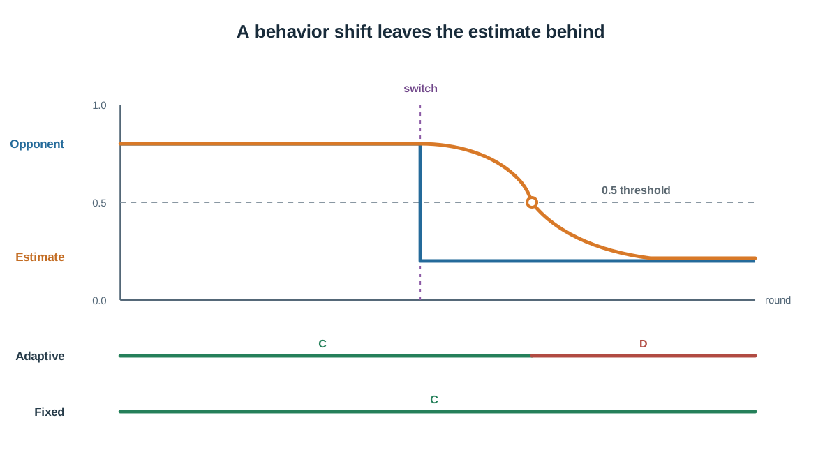
The script above already contains the shift. Set switch_at=250 and p_second=0.2, and the adaptive agent pays a switching cost: for several steps after the change, it keeps playing the stale best response while the estimate catches up.
Push the switch earlier and watch the advantage shrink or reverse:
for switch in (50, 100, 250, 400):
    rng = random.Random(7)
    stream = list(opponent_stream(500, switch, 0.8, 0.2, rng))
    a, f, err = run(stream)
    print(f"switch={switch:>3}  adaptive={a}  fixed={f}  diff={a - f:+d}")
When the switch happens early, the fixed response never gets a clean stationary phase to lock onto, and the adaptive agent's lag is amortized over more of the episode. When the switch happens late, the fixed response has already banked its advantage and the adaptive agent cannot recover.
The minimal fix is a decayed or windowed frequency estimate: weight recent observations more heavily so the estimate tracks a moving target.
def run_decayed(stream, decay=0.95, warmup=50):
    est = 0.5
    fixed_action = None
    coop_count, total = 0, 0
    adaptive_payoff, fixed_payoff = 0, 0
    for t, opp in enumerate(stream):
        adaptive_action = best_response(est)
        if fixed_action is None and total >= warmup:
            fixed_action = best_response(coop_count / total)
        fixed_action = fixed_action or best_response(0.5)
        adaptive_payoff += PAYOFF[(adaptive_action, opp)]
        fixed_payoff += PAYOFF[(fixed_action, opp)]
        obs = 1.0 if opp == "C" else 0.0
        est = decay * est + (1 - decay) * obs
        coop_count += (opp == "C")
        total += 1
    return adaptive_payoff, fixed_payoff
Decay trades responsiveness against estimate variance. A high decay rate tracks slowly and stays stable; a low decay rate reacts fast but bounces on noise. There is no free setting — you are choosing which failure mode you can tolerate.
Knowledge check
Check your understanding
Answer this question before you continue.
Failure Modes and Debugging Signals
| Symptom | Likely cause |
|---|---|
| Identical payoff for both agents | The opponent stream was not actually shared, or the seed was reset between runs. |
| Adaptive agent never improves | The frequency update is applied after the decision instead of before, or the estimate is reset each step. |
| Payoff advantage flips between seeds | The episode is too short relative to the switching cost; the result is noise. |
| Prediction error stays flat while payoff rises | The agent is exploiting a payoff asymmetry, not tracking the opponent. |
The last row is the one that fools people. A rising payoff feels like success. But if prediction error is flat, the model is not doing the work — the payoff matrix is. Change the matrix and the advantage evaporates.
Tip: Log prediction error in every run, not just the final one. The trajectory of the error tells you whether the model is converging, oscillating, or tracking a moving target.
What This Model Cannot Do
Use a frequency estimate when the opponent's policy is roughly stationary, the action space is small, and the cost of a wrong prediction is bounded. Those three conditions cover a surprising amount of practical ground.
Do not use it when:
- The opponent conditions on your actions. A frequency estimate ignores state and history, so it cannot represent conditional strategies like tit-for-tat.
- The action space is large. One number per action stops being cheap when there are thousands of actions.
- The opponent is itself learning and adapting. Your estimate chases a target that is chasing you.
The gap is explicit: a frequency estimate ignores state, history, and reciprocity. It is a marginal distribution, not a policy. Richer representations — policy embeddings, recursive opponent models, uncertainty-aware models — exist precisely because the marginal distribution is not enough when the opponent's behavior depends on context.
Extend the Experiment
One concrete next modification: add a second opponent type with a different action distribution and test whether the adaptive agent's advantage holds across both.
for p_c in (0.2, 0.5, 0.8):
    rng = random.Random(7)
    stream = list(opponent_stream(500, switch_at=250, p_first=p_c, p_second=1 - p_c, rng=rng))
    a, f, err = run(stream)
    print(f"p_first={p_c}  adaptive={a}  fixed={f}  diff={a - f:+d}")
Then sweep the switch point and plot payoff difference against how late the change occurs. Compare a fixed decay rate against a windowed estimate to see how the responsiveness-variance tradeoff shows up in the numbers. Record prediction error alongside payoff in every run, because the two together are what make the result interpretable.
The decision rule to carry forward: an opponent model is only worth its complexity when its estimate tracks a real, stable signal. The way to know is to measure prediction error next to payoff — not payoff alone. When the opponent is itself learning, the frequency estimate stops being sufficient, and the next experiment in this track takes up that case directly.
Knowledge check
Final check
Finish the article by checking the ideas you just learned.
References
Build a stronger RL mental model
Use structured resources to connect equations, algorithms, and observable agent behavior.


