
Update a Bayesian Model of an Opponent’s Actions
Frequency counting answers with a single number and no error bar. It cannot tell you how much evidence you actually have, and it has no place to put what…

Key topics
Four identical actions in a row. Is that a tendency or a coincidence?
Frequency counting answers with a single number and no error bar. It cannot tell you how much evidence you actually have, and it has no place to put what you already believed before the first observation. The fix is to stop tallying actions and start maintaining a belief over the opponent's action distribution. That belief has a two-line update rule, a predictive probability you can compute on paper, and exactly one assumption holding it together.
This article assumes you already accept that predicting another learner can improve adaptation. The question here is narrower and more mechanical: how do you represent that prediction as a probability distribution, and how does it change when new actions arrive?
What You Are Actually Estimating
Before any notation, fix the target. You are not modeling a sequence of decisions. You are modeling the opponent as a fixed conditional distribution over actions — a single object that generates every action it takes.
The unknown quantity is the parameter vector of that distribution, not the next action. This distinction matters because it changes what your belief is about. The opponent's action is sampled; the parameter is inferred. You observe the sample, and you reason backward to the thing that produced it.
Two assumptions make this tractable, and you should name them now because the last section dismantles the first:
- Stationarity. The opponent's action distribution does not change over the horizon you care about.
- Independence. The opponent's strategy does not depend on your behavior.
Both are strong. Both are also the reason the update stays closed-form and cheap. Hold that trade in mind.
Notation and the Categorical Likelihood
Let the opponent choose from an action set of size . Index actions through . The parameter vector is
Each is the probability the opponent plays action . The constraint is not decoration — it defines the space the parameter lives in, and the prior you choose later has to respect it.
The likelihood of a single observed action is just the matching entry:
For a sequence of independent actions, the likelihood is a product:
where is the number of times action appeared. That last step is the important one: the product collapses into counts per action. The likelihood depends only on , not on the order in which the actions arrived.
Order-independence is a real modeling commitment, not a convenience. It is precisely what stationarity buys you. If the opponent's distribution were drifting, the order would carry information, and collapsing to counts would throw it away. For now, assume it does not drift. This count vector is the sufficient statistic — everything the data can tell you about is already in it.
The multinomial distribution is the general form for draws; the categorical is the single-draw case. You will use the categorical likelihood above and the multinomial when you batch observations.
Knowledge check
Check your understanding
Answer this question before you continue.
Why the Dirichlet Prior Fits
You need a prior over . The Dirichlet distribution is the natural choice, for two reasons.
First, its support is the simplex — the same constrained space lives in. The prior never assigns probability mass to parameter vectors that violate . A Gaussian prior would, and you would spend effort correcting for it.
Second, each Dirichlet parameter behaves like a prior observation count. Write the prior as
with concentration parameters , each . Read as "how many times I have already seen action before collecting any data." A uniform prior with all is a weak belief. A prior with and the rest at is a confident claim that action dominates, and it will resist contradicting data.
The third reason is conjugacy: the Dirichlet is the conjugate prior for the categorical and multinomial likelihoods. Multiply the two and you get another Dirichlet. That is what keeps the update closed-form.
Note: A bad prior is not wrong. It is slow to be corrected. If you set high and the opponent actually favors action , your posterior will lag reality for many observations. That lag is the visible cost of an overconfident prior, and it shows up as delayed adaptation.
Knowledge check
Check your understanding
Answer this question before you continue.
Deriving the Posterior Update
Now the Bayes step, done explicitly so you can see where the addition comes from.
The posterior is likelihood times prior, normalized:
Substitute both pieces. The likelihood contributes and the prior contributes . Multiply them — the exponents add:
That is a Dirichlet with updated parameters. Name them:
The posterior concentration equals the prior concentration plus the observed count, per action. That is the whole update. No iteration, no gradient, no tuning.
The normalizing constant is a ratio of beta functions, , and you almost never compute it for prediction — the proportionality is enough.
Read the update as a ledger. Prior counts on one side, evidence counts on the other, sum them. The posterior mean is
Warning: If you set some , the prior assigns zero mass to that action, and if you never observe it, the posterior keeps it at zero forever. No amount of other evidence revives it. That is a modeling choice with permanent consequences — avoid zero concentrations unless you genuinely mean "impossible."
Knowledge check
Check your understanding
Answer this question before you continue.
Worked Example: Three Actions, Six Observations
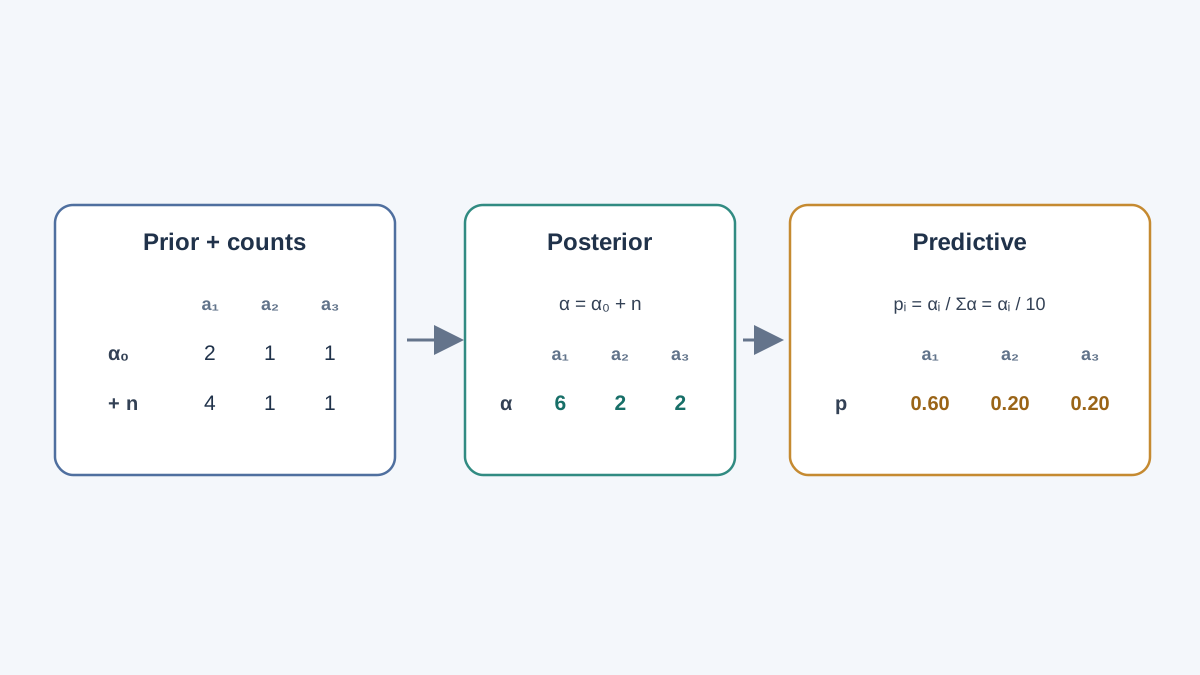
Let . Choose a deliberately weak, slightly asymmetric prior so you can see its influence without it dominating:
The opponent plays the sequence: action 1, action 3, action 1, action 1, action 2, action 1. Tally the counts:
Apply the update by addition:
The posterior mean is divided by its total, which is :
Compare that against the raw empirical frequency, . The prior pulled action 1 down from to and nudged the others up. That pull is the prior's weight showing through — small here, because the prior total is against observations.
The posterior predictive probability of the next action is the probability of that action given the data, integrating over your uncertainty about :
For this model, the predictive mean equals the posterior mean. So the next-action prediction is .
Now add a second round. Suppose the opponent plays action 2 four more times. The new counts are , and the posterior becomes
The prior's pull has shrunk. With observations against a prior total of , the data now dominates. That is the behavior you want: weak priors get out of the way fast, strong priors do not.
| Action | Prior | Observed | Posterior | Posterior mean |
|---|---|---|---|---|
| 1 | 2 | 4 | 6 | 0.60 |
| 2 | 1 | 1 | 2 | 0.20 |
| 3 | 1 | 1 | 2 | 0.20 |
Knowledge check
Check your understanding
Answer this question before you continue.
Reading Uncertainty, Not Just the Mean
The mean is the headline. The spread is the story.
The total concentration controls how peaked the posterior is. Two opponents can share an identical posterior mean with very different credible intervals. If one posterior is and another is , both have mean — but the first is a confident belief and the second is a shrug.
Here is the part that trips people up. For this model, the one-step posterior predictive probabilities are exactly the posterior mean, regardless of concentration. Both posteriors above predict the next action with the same vector. Concentration does not change that vector.
What concentration changes is your uncertainty about the parameters, and that matters for decisions in a different way. A narrow posterior means you are confident the opponent's true is near . A wide posterior means the true could be anywhere in a broad region — the mean is just its center of mass. If you exploit the mean aggressively, you are betting that the true distribution is close to it. That bet is cheap when the posterior is narrow and expensive when it is wide.
So the honest statement is this: the predictive vector tells you what to expect on the next draw; the posterior width tells you how much to trust that expectation when you act on it. Risk-sensitive planning and value-of-information calculations use the width. A greedy action selection that only reads the predictive vector ignores it.
Common mistake: Assuming that a wide posterior produces a "flatter" predictive distribution. It does not. A wide posterior centered on the same mean produces the same one-step predictive. The width shows up in multi-step predictions, in risk, and in how much a single new observation can move your belief — not in the next-action probability vector.
When the Stationary Assumption Breaks
Everything above rests on the opponent's distribution being fixed. Here is what happens when it is not.
Policy drift. The opponent's true changes while your posterior keeps accumulating counts. Old evidence is silently weighted as if it were current. Your model becomes a historian of a strategy that no longer exists.
Strategic response. The opponent conditions on your behavior. This violates independence directly: the likelihood assumes the opponent's action does not depend on yours, and now it does. The model is misspecified, and no amount of data fixes a wrong likelihood.
The diagnostic signature is specific and worth memorizing: the posterior becomes confidently wrong. It narrows and centers on a stale value. This is worse than being uncertain, because a narrow wrong belief drives aggressive exploitation of a pattern that has already changed. Uncertainty keeps you cautious; false confidence gets you punished.
Mitigations exist, each with a cost:
| Approach | Mechanism | Cost |
|---|---|---|
| Exponential forgetting | Decay old counts by a factor each step | Trades sample efficiency for responsiveness |
| Windowed counts | Keep only the last observations | Discards potentially useful history |
| Change-point / switching model | Explicitly model regime changes | More parameters, more inference |
Each buys responsiveness by giving up the statistical efficiency that came from pooling all history. That is the real trade: the stationary model is sample-efficient precisely because it trusts old data, and that trust is what breaks under drift.
Common mistake: Reaching for a forgetting factor before confirming the opponent is actually non-stationary. If the opponent is a fixed scripted policy, decayed counts just add noise to a model that was already correct. Diagnose drift first.
Where This Fits in a Multi-Agent Loop
The posterior is a belief state. It summarizes what you know about the opponent in a fixed-size vector, and you feed it into planning or value estimation as an input feature. It does not replace your policy; it informs it.
Keep the prediction problem and the control problem separate. A good posterior does not automatically produce a good response — that is a second design decision about how aggressively to exploit what you believe.
And watch the coupling. If your policy exploits the posterior hard, you change the opponent's behavior, which invalidates the model you are exploiting. This is the loop that turns a clean Bayesian update into a moving target, and it is the reason opponent modeling in multi-agent reinforcement learning is harder than the single-agent case.
Natural extensions follow from here: condition the model on state, condition it on the opponent's information set, or replace the fixed prior with a hierarchical one over opponent types so the model can represent "this is one of several kinds of player" rather than one fixed distribution.
The Decision Rule
Use the Dirichlet-categorical model when the opponent is plausibly fixed within the horizon you care about. The update is two lines, the prediction is a division, and the uncertainty comes for free.
Switch to decayed counts or a switching model the moment you see a narrow posterior that keeps mispredicting. That symptom — confidence without accuracy — is the signal that stationarity has failed.
Here is your next move. Implement the update in a few lines: keep a count vector, add observations, divide by the total. Run it against a scripted opponent and confirm the posterior converges to the true distribution. Then run it against an opponent that changes strategy halfway through and watch the posterior lie to you with a straight face. The gap between those two runs is the entire lesson.
Knowledge check
Final check
Finish the article by checking the ideas you just learned.
References
Build a stronger RL mental model
Use structured resources to connect equations, algorithms, and observable agent behavior.


