
Test Prior Sensitivity in a Bayesian Opponent Model
Same opponent. Same six observed actions. Same code. Two different decisions — because the prior changed.

Key topics
Same opponent. Same six observed actions. Same code. Two different decisions — because the prior changed.
That is the whole exercise. You will freeze the observation vector, vary only the Dirichlet prior, and watch the posterior, the predictive distribution, the uncertainty, and the final decision move. If the decision flips, you have found the mechanism this exercise exists to expose: a predictive mean is not a belief, and a belief is not a decision until you attach a loss to it.
This is a controlled experiment, not a formula drill. The goal is to interpret uncertainty, not to memorize the update rule.
What This Exercise Is Actually Testing
You already know the prerequisite machinery: a Dirichlet prior over a categorical action distribution, plus observed counts, yields a Dirichlet posterior with parameters alpha + counts, and the posterior predictive for the next action is the normalized posterior mean. I am not going to re-derive that here. If the conjugacy step feels shaky, go back to the update tutorial first — this exercise assumes it.
What you are testing here is narrower and more uncomfortable:
- One fixed action sample. It never changes.
- At least two stated Dirichlet priors.
- Posterior parameters, posterior predictive probabilities, and an uncertainty measure for each.
- A decision rule with asymmetric loss, so the threshold is not 0.5.
- A printed comparison showing whether the decisions diverge.
The constraint is the point. Because the counts are frozen, every difference in the output is attributable to the prior. No confounds, no sampling noise, no seed.
Note: Standard library only. No NumPy, no SciPy, no sampling library. The arithmetic is small enough to write by hand, and writing it by hand is what makes the pseudo-count mechanism visible instead of hidden behind a
dirichlet.rvs()call.
Success is observable: your program prints the priors, the observations, the posterior parameters, the predictive probabilities, an uncertainty comparison, and the threshold-based decision for each prior — and the decisions are not all the same.
Set Up the Model and the Three Priors
Three opponent actions: pass, call, raise. Three categories means the Dirichlet is genuinely multivariate — you cannot fall back on Beta intuition, and the concentration parameter has to be reasoned about as a vector plus a total.
The fixed observation vector is deliberately small:
ACTIONS = ["pass", "call", "raise"]
COUNTS  = [1, 4, 1]   # 6 observations total
Six observations. Small enough that the prior still has visible weight. This is the regime where prior sensitivity is real rather than a rounding artifact. With 600 observations, almost any reasonable prior washes out and the exercise teaches nothing.
Now the priors. Each is a length-3 vector of positive concentration parameters.
PRIORS = {
    "A_flat":        [1.0, 1.0, 1.0],   # no idea what this opponent does
    "B_call_heavy":  [1.0, 12.0, 1.0],  # "this opponent mostly calls"
    "C_contrarian":  [8.0, 1.0, 8.0],   # mildly concentrated, disagrees with data
}
Prior A is near-flat: total concentration 3, so it behaves like three pseudo-observations spread evenly. It says "I have no idea."
Prior B is concentrated on call: total concentration 14, with 12 of those pseudo-counts sitting on call. It says "I have seen this opponent call a lot, and I believe it."
Prior C is the interesting one. It is mildly concentrated — total 17 — and it disagrees with the data, which is heavy on call. This is where you see the posterior being pulled rather than merely nudged.
The single number that controls prior resistance is the sum of the alpha parameters. That sum behaves like a number of pseudo-counts. Compare it against N, the number of real observations. When sum(alpha) is comparable to N, the prior is still steering. When sum(alpha) is tiny relative to N, the data drives. Everything else is detail.
Write the Posterior and Predictive Calculation
Here is the smallest runnable program that produces the core numbers. Read it as arithmetic, not as architecture.
ACTIONS = ["pass", "call", "raise"]
COUNTS  = [1, 4, 1]

PRIORS = {
    "A_flat":       [1.0, 1.0, 1.0],
    "B_call_heavy": [1.0, 12.0, 1.0],
    "C_contrarian": [8.0, 1.0, 8.0],
}

def posterior_alpha(alpha, counts):
    return [a + n for a, n in zip(alpha, counts)]

def predictive(alpha, counts):
    post = posterior_alpha(alpha, counts)
    total = sum(post)
    return [p / total for p in post]

def total_concentration(alpha, counts):
    return sum(posterior_alpha(alpha, counts))

for name, alpha in PRIORS.items():
    post = posterior_alpha(alpha, COUNTS)
    pred = predictive(alpha, COUNTS)
    conc = total_concentration(alpha, COUNTS)
    print(f"--- {name} ---")
    print(f"  prior alpha      : {alpha}  (sum={sum(alpha)})")
    print(f"  counts           : {COUNTS}  (N={sum(COUNTS)})")
    print(f"  posterior alpha  : {post}  (sum={conc})")
    print(f"  predictive       : {[round(p, 4) for p in pred]}")
Two functions carry the whole mechanism.
posterior_alpha is elementwise addition. That is the entire conjugacy payoff: the Dirichlet prior plus categorical counts yields a Dirichlet posterior, and the update is alpha_k + n_k. No integration, no normalization constant, no sampling. This is why the Dirichlet-categorical pair is the default choice for opponent action models — the update is cheap enough to run inside a game loop.
predictive normalizes the posterior parameters. The posterior predictive probability for action k is (alpha_k + n_k) / (sum(alpha) + N), which is exactly the posterior mean of the categorical parameter vector. Implement it directly; do not reach for a library.
Run it and watch the pseudo-counts turn into probabilities. Prior A, with total concentration 3, gets dragged almost entirely to the data: call lands near 0.56. Prior B, with total concentration 14 and 12 pseudo-counts on call, resists: call lands near 0.80. Prior C, with 16 pseudo-counts split evenly between pass and raise, fights the data and pulls call down relative to the flat prior.
Same six observations. Three different predictive distributions. That is the first half of the lesson.
Knowledge check
Check your understanding
Answer this question before you continue.
Quantify the Uncertainty, Not Just the Mean
Here is the failure mode this section exists to catch: two priors can produce similar predictive means while carrying very different uncertainty. If you print only the mean, you cannot tell a confident claim from a shrug.
The Dirichlet gives you a closed-form variance per category. No sampling required:
def posterior_variance(alpha, counts):
    post = posterior_alpha(alpha, counts)
    total = sum(post)
    return [p * (total - p) / (total * total * (total + 1)) for p in post]
The denominator depends on the total concentration, not just the per-action parameter. Get that wrong and you produce plausible-looking numbers that mean nothing — a classic silent bug in this kind of code.
Print the variance (or its square root) side by side with the predictive means:
for name, alpha in PRIORS.items():
    pred = predictive(alpha, COUNTS)
    var  = posterior_variance(alpha, COUNTS)
    conc = total_concentration(alpha, COUNTS)
    print(f"--- {name} ---  total concentration = {conc}")
    for a, p, v in zip(ACTIONS, pred, var):
        print(f"  {a:5s}  p={p:.4f}  var={v:.6f}  sd={v**0.5:.4f}")
The interpretation rule is blunt: a high predictive probability from a low-concentration posterior is a weak claim, not a strong one. Prior A's call probability of ~0.56 comes with a wide spread because the total concentration is only 9. Prior B's call probability of ~0.80 comes with a tighter spread because the total concentration is 20. The mean moved up and the uncertainty shrank — those are two separate facts, and only one of them is visible if you print the mean alone.
Total concentration is a useful scalar confidence proxy, but be honest about what it does and does not capture. It tells you how much evidence — real plus pseudo — is behind the posterior. It does not tell you whether that evidence is relevant. A concentrated prior built on stale assumptions gives you a confident posterior for the wrong reason.
Knowledge check
Check your understanding
Answer this question before you continue.
Turn Probabilities Into a Decision With Asymmetric Loss
A probability is not a decision. To get a decision, you need a loss.
Define a concrete task: the agent must decide whether to commit to a counter-action that beats call. Being wrong in one direction is more expensive than being wrong in the other. Say a false positive — committing when the opponent will not call — costs C_fp = 3. A false negative — failing to commit when the opponent will call — costs C_fn = 1.
The decision flips at the point where expected loss is equal:
p * C_fn = (1 - p) * C_fp
p = C_fp / (C_fp + C_fn)
With C_fp = 3 and C_fn = 1, the threshold is 3 / 4 = 0.75. Commit only when the predictive probability of call exceeds 0.75.
C_FP, C_FN = 3.0, 1.0
THRESHOLD = C_FP / (C_FP + C_FN)   # 0.75

for name, alpha in PRIORS.items():
    pred = predictive(alpha, COUNTS)
    p_call = pred[ACTIONS.index("call")]
    decision = "COMMIT" if p_call > THRESHOLD else "HOLD"
    print(f"{name:14s} p(call)={p_call:.4f}  threshold={THRESHOLD:.2f}  -> {decision}")
Now look at what happens. Prior A gives p(call) ≈ 0.56, below 0.75 — HOLD. Prior B gives p(call) ≈ 0.80, above 0.75 — COMMIT. Prior C gives p(call) ≈ 0.35 — HOLD, and not even close.
Identical counts. Opposite decisions. The prior did that.
Common mistake: Setting a symmetric loss. With
C_fp = C_fn, the threshold is exactly 0.5, and in that regime the prior choice frequently does not change the decision. That is precisely why prior sensitivity is easy to miss: the default loss function hides it. Move the threshold away from 0.5 and the fragility becomes visible.
Knowledge check
Check your understanding
Answer this question before you continue.
Read the Output: Where the Decisions Diverge
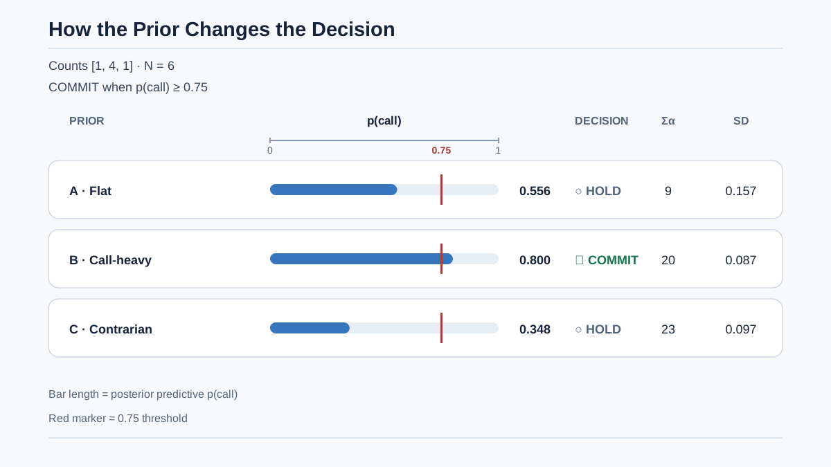
Here is the full printed block for each prior, condensed:
--- A_flat ---        prior sum=3   posterior sum=9
  p(call)=0.5556   var=0.0247   sd=0.1571
  threshold=0.75   -> HOLD

--- B_call_heavy ---  prior sum=14  posterior sum=20
  p(call)=0.8000   var=0.0076   sd=0.0872
  threshold=0.75   -> COMMIT

--- C_contrarian ---  prior sum=17  posterior sum=23
  p(call)=0.3478   var=0.0094   sd=0.0970
  threshold=0.75   -> HOLD
Trace the divergence step by step. The counts are identical. The posterior parameters differ because the priors differ. The predictive probabilities differ because the posterior parameters differ. The decisions differ because the predictive probabilities straddle the threshold.
The exact step where the runs separate is the posterior concentration. Prior A's total concentration is 9, so the six observations dominate and call sits near the empirical rate. Prior B's total concentration is 20, so the 12 pseudo-counts on call hold the estimate up. Prior C's total concentration is 23, and its pseudo-counts actively fight the data.
Three regimes fall out of this:
| Regime | Condition | Behavior |
|---|---|---|
| Prior-dominated | sum(alpha) >> N | Posterior barely moves; decision reflects the prior |
| Data-dominated | sum(alpha) << N | Posterior tracks the empirical counts; prior is irrelevant |
| Contested middle | sum(alpha) ≈ N | Decision is genuinely fragile; small changes flip it |
This exercise lives in the contested middle on purpose. That is where decisions are made and unmade by assumptions you did not examine.
Why this matters in multi-agent RL: an opponent model that is confident for the wrong reason produces a confident wrong counter-strategy. The confidence is invisible if you only print the mean. You will commit to a counter-action, lose, and blame the policy — when the real fault was a prior you never questioned.
Warning: This model assumes a stationary opponent. A decision that looks stable here can still be wrong the moment the opponent adapts to your behavior. Prior sensitivity is one failure axis; non-stationarity is a separate one, and they compound.
Knowledge check
Check your understanding
Answer this question before you continue.
Failure Modes and Debugging Signals
Each wrong output points at a specific bug. Learn the signals.
Predictive probabilities that do not sum to 1. Usually a missing normalization, or a counts vector whose length does not match the action list. Check that zip(alpha, counts) is not silently truncating to the shorter sequence.
Identical output for both priors. Two causes. Either the alpha sums do not actually differ (you edited the wrong dictionary), or N is so large that the prior cannot matter. Shrink the observation count until the priors separate.
A decision that never flips. The threshold is probably at or near 0.5, or the prior difference is too small relative to the data. Widen the loss asymmetry or increase the prior concentration gap.
Variance computed with the wrong denominator. The Dirichlet variance depends on the total concentration, not just the per-action parameter. Using p * (1 - p) / total instead of p * (total - p) / (total * (total + 1)) produces numbers that look reasonable and are wrong. This is the most dangerous bug in the exercise because nothing crashes.
Treating a high posterior mean as high confidence. The most common conceptual error, and the one the uncertainty section exists to catch. A mean of 0.80 from a total concentration of 5 is a rumor. A mean of 0.80 from a total concentration of 500 is a fact. Same number, different world.
Modify the Experiment
Do not rerun the same script. Change one variable and watch the decision boundary move.
Sweep the observation count. Hold both priors fixed and grow COUNTS from 1 to 50 total observations, printing the decision at each step. Find the crossover point where the prior stops changing the outcome. That number is the answer to the real question: how much evidence do I need before I can stop worrying about my prior?
Sweep the loss ratio instead. Hold the posterior fixed and vary C_fp / C_fn. The same posterior produces different decisions under different operational costs. The prior is not the only lever — the loss is the other one, and it is often the one you control.
Add a fourth action category. Watch how the extra dimension changes the concentration dynamics. With more categories, the same total concentration spreads thinner, and the posterior becomes less certain per category.
The interpretation target: for your own numbers, state how many observations are needed before the prior choice stops changing the decision. If you cannot state that number, you have not finished the exercise.
What to Carry Forward
Before you trust an opponent model's prediction, check two numbers: the posterior concentration and the loss asymmetry. Those two — not the predictive mean alone — determine whether the prior is still steering your decision.
The predictive mean tells you what the model expects. The concentration tells you how much it should be believed. The loss tells you whether believing it is worth acting on. Miss any one of the three and you will make a confident decision for a reason you cannot defend.
Your next move: take your own action data from a repeated interaction, run the observation-count sweep, and find the point where your prior stops mattering. That crossover point is the boundary between guessing and knowing — and it is different for every opponent you will ever model.
Knowledge check
Final check
Finish the article by checking the ideas you just learned.
References
Build a stronger RL mental model
Use structured resources to connect equations, algorithms, and observable agent behavior.


