
Multi-Agent Reinforcement Learning Explained: What Changes When Other Agents Learn Too?
Single-agent RL treats the environment as a fixed target. Add a second learning agent, and the target starts moving.

Key topics
Single-agent RL treats the environment as a fixed target. Add a second learning agent, and the target starts moving.
If you have worked through Markov decision processes and policy optimization, you inherited a quiet assumption: the environment's transition and reward functions are stable objects, and your agent is the only thing changing its behavior. That assumption props up your value estimates, your replay buffers, and your convergence guarantees. Multi-agent reinforcement learning pulls the assumption out and asks what still stands.
The Single-Agent Assumption That Breaks First
In a single-agent MDP, the world obeys a fixed contract. The transition function maps states and actions to next states with probabilities that never change. The reward function is static. Your policy improves, but the environment does not adapt to your improvements.
The moment a second learning agent enters, that contract changes shape.
The environment now transitions on the joint action of every agent, not on your action alone. If two agents act, the next state depends on both choices. That alone is manageable—you could treat the other agent's action as part of the environment's randomness. But the other agent is not random noise. It is learning. Its policy is changing, and the transition dynamics you experience are changing with it.
From your perspective, the environment has become non-stationary. The Markov property you relied on—that the next state depends only on the current state and action—still holds at the level of the full system. But you do not observe the full system. You observe your own state, and the dynamics governing that state shift whenever your neighbor updates its policy.
This is the moving-target problem. In single-agent RL, you chase a fixed optimum. In multi-agent reinforcement learning, every agent chases an optimum that other agents keep relocating.
Knowledge check
Check your understanding
Answer this question before you continue.
One Timestep, Seen Through Every Agent's Eyes
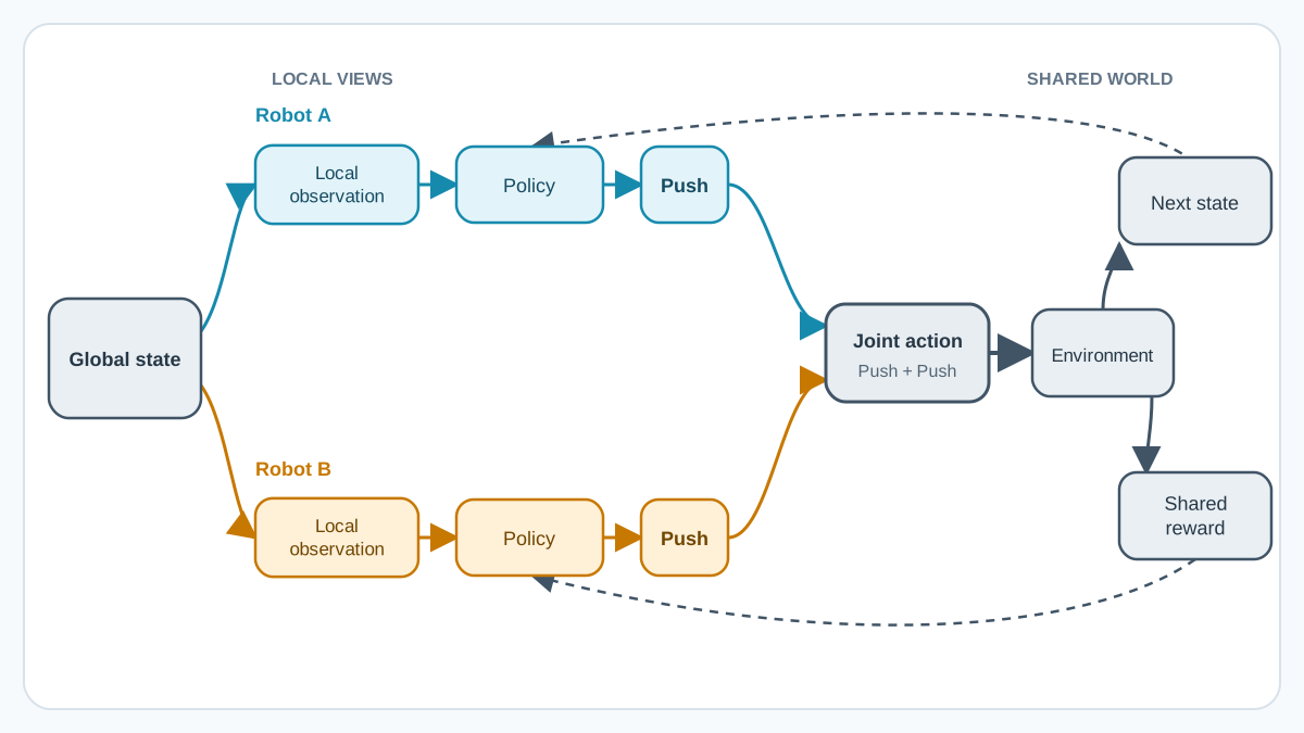
To see why this matters, trace a single step in a concrete setting: two robots moving a crate together. Each robot pushes from one side, and the crate moves only when both push in compatible directions.
At time t, the global state includes both robot positions, the crate position, and its velocity. Neither robot sees all of it. Robot A observes its own position and the crate's position relative to it. Robot B observes the same kind of local information from its side. Each robot's policy maps its local observation to a push direction.
The joint action—both pushes—determines the next state. If the pushes align, the crate moves and the team earns a shared reward. If they oppose, the crate barely moves and the reward is small.
Now update both policies. Robot A's update assumes Robot B's behavior is fixed. Robot B's update assumes the same about A. Both assumptions are false. At time t+1, each robot faces dynamics that shifted because the other agent changed its push strategy. The local observation also hides information: Robot A cannot directly see what B is about to do, so part of the state that determines the next transition is invisible to it.
This one step contains the entire field's difficulty. Joint actions create hidden dependence. Learning changes the other policy. Local observations hide relevant state. And when the crate finally arrives, the shared reward does not say which robot pushed effectively and which interfered. That last problem—credit assignment—is invisible in single-agent RL because there is only one contributor to blame or praise.
Knowledge check
Check your understanding
Answer this question before you continue.
Why Non-Stationarity Is Not Just Noise
It is tempting to file non-stationarity under "environmental stochasticity" and move on. That would be a mistake.
Noise is benign because it is stable. A noisy transition function has fixed statistics; enough samples average it out. Non-stationarity is different: the statistics themselves drift. The experience distribution you collect this episode becomes stale the moment another agent improves its policy. Your replay buffer fills with data from a world that no longer exists.
The consequence is structural, not merely inconvenient. Convergence guarantees from single-agent RL evaporate because they depend on a stationary target. When your neighbor's policy shifts, the optimal policy for you shifts too. There may be no fixed point at all, or the fixed point may be unreachable by agents that keep reacting to each other's last move.
Picture two archers shooting at targets mounted on each other's backs. Every time one improves her aim, the other's target moves. Neither can settle into a stable solution by optimizing against a snapshot of the other's behavior, because the snapshot is outdated by the time it is used.
Common mistake: Treating every unstable training run as a MARL phenomenon. Implementation bugs, sparse rewards, and poor exploration also produce oscillating curves. Non-stationarity is the right diagnosis only when you have controlled for the ordinary failure modes.
Knowledge check
Check your understanding
Answer this question before you continue.
Cooperation, Competition, and the Mixed Middle
Before choosing any method, classify the relationship between agents. The reward structure defines what problem you are actually solving.
Cooperative settings give agents aligned rewards. A team succeeds or fails together; one agent's gain is not another's loss. Think of robots moving a heavy object jointly, or traffic signals coordinating to reduce intersection congestion. The design question becomes how agents should share information and divide credit.
Competitive settings are zero-sum: one agent's reward is exactly another's loss. Chess, poker, and pursuit-evasion games fit here. Your gain is my loss, so my optimal strategy must account for your incentive to defeat me.
Mixed cooperative-competitive settings combine both. Teams align internally while opposing externally. The classic simple_tag environment makes this concrete: a team of chasers pursues evaders, with chasers collectively rewarded for contact and the touched evader penalized by the same amount. Within each team, agents cooperate; between teams, they compete.
The relationship type dictates your method family. Cooperative problems reward information sharing and coordinated exploration. Competitive problems demand opponent modeling—predicting what the other agent will do, not just reacting to what it did. Mixed problems require both, plus a mechanism for balancing internal cooperation against external competition.
Knowledge check
Check your understanding
Answer this question before you continue.
What Each Agent Actually Sees and Decides
In most MARL settings, no agent observes the full global state. Each holds a local, partial observation: its own position, velocity, and relative information about nearby agents and obstacles. This partial observability is not an implementation detail; it is the realistic condition of almost any deployed system.
Execution is typically decentralized. Each agent's policy maps its own observation to its own action, with no central controller consulting the full state at decision time. This structure is a practical necessity when agents are physically distributed or when communication is expensive—not merely a theoretical preference.
Training is a separate question. Centralized training with decentralized execution (CTDE) is the pattern that dominates modern methods: agents execute with local information, but training has access to global state and joint actions. A centralized critic can observe everything, which helps it evaluate actions in a way that accounts for other agents' behavior. The policy remains local; only the learning signal is global.
Parameter sharing adds another wrinkle. Many agents can reuse a single policy network, each acting from its own observation. Shared parameters reduce memory and sample complexity dramatically, and agents remain behaviorally distinct because their observations differ. The shared policy is a common brain with different sensory inputs.
Choosing a Method Family by Problem Structure
The method families below are responses to specific failures. Match the failure to the fix, and check the prerequisites before committing.
| Problem structure | Method family | What it needs | What it does not solve |
|---|---|---|---|
| Independent learners facing non-stationarity | Centralized critic (CTDE) | Global state and joint actions available during training | Distributed training with no central information channel |
| Cooperative team with shared rewards | Value decomposition | Team-level value signal plus a factorization structure | Competitive dynamics where agents have opposing goals |
| Competitive or mixed settings | Opponent modeling | Ability to observe or infer other agents' behavior | Fully cooperative tasks where modeling adds little |
| Many agents with large joint action spaces | Parameter sharing, factorization, or communication protocols | Structural symmetry or a communication channel | Asymmetric roles with no shared structure |
Centralized critics help overcome non-stationarity by giving each agent's value estimate access to other agents' actions, removing some of the hidden variance. But they are not a default fix: they require global information during training, and their input space grows with the number of agents.
Value decomposition targets credit assignment in cooperative teams by learning how to split team value among individual agents. It assumes the team's value can be factored into per-agent contributions—an assumption that fails when agents interact in ways that cannot be decomposed.
Opponent modeling matters whenever interests conflict. An agent that models its opponent's policy can anticipate behavior rather than react to it. But it introduces a recursive problem: if I model you, and you model me modeling you, where does the regression end?
Note: CTDE, parameter sharing, value decomposition, and opponent modeling are not mutually exclusive. Practical systems often combine them. The question is which failure dominates your problem, not which label you prefer.
Where to Go Next
My rule for choosing a MARL direction: classify your problem by relationship type and observability before you look at any algorithm.
Ask whether rewards align, oppose, or mix. Ask what each agent can observe at execution time and what training can access. Those two answers eliminate most method families immediately.
Then make the moving-target problem visible with a diagnostic experiment. Take a simple two-agent environment you know well, train both with independent Q-learning, and measure four things:
- Each agent's action frequencies over time, to see whether policies drift.
- Episode returns, to see whether performance oscillates or collapses.
- Each agent's performance against a frozen checkpoint of the other agent's policy, to isolate the effect of the other agent's updates.
- The difference between learning from fresh experience versus replayed experience, to detect stale data.
If action frequencies drift while the frozen-checkpoint evaluation stays stable, you have evidence of a moving target. If the frozen-checkpoint evaluation also degrades, suspect implementation bugs, sparse rewards, or partial observability instead.
That instability is not always a bug in your implementation. Sometimes it is the moving-target problem made visible.
Multi-agent reinforcement learning is not RL with more agents. It is RL where the environment learns back.
Knowledge check
Final check
Finish the article by checking the ideas you just learned.
References
Research updated Sep 9, 2026


