
Test How Planning Horizon Changes Decisions Under Model Error
A planner can be confidently wrong. Give it a slightly inaccurate model and a long enough horizon, and it will walk off a cliff while reporting that the…

Key topics
A planner can be confidently wrong. Give it a slightly inaccurate model and a long enough horizon, and it will walk off a cliff while reporting that the cliff was the best move on the board.
That is the failure this experiment is built to expose. You already know the theory: small one-step model errors compound across imagined rollouts, and a longer planning horizon can quietly turn foresight into fiction. Knowing it in principle is not the same as watching it happen in output you can print, measure, and vary on demand.
So we are going to build the smallest possible stress test. One tiny gridworld. One dial for planning horizon. One dial for model error. Two measurements: what the planner predicted would happen, and what actually happened when it acted. The gap between those two numbers is the whole lesson.
By the end you will have a runnable script and a decision rule: horizon is a complexity dial, not a quality dial, and the only honest way to set it is to measure predicted versus true outcomes under controlled error.
What This Experiment Is Actually Testing
Before any code, get the task and the variables straight. Confusion here wastes the whole run.
The task is a small deterministic gridworld with three features: a fixed start state, a goal that pays a reward, and a pit that pays a large penalty. The true dynamics are known exactly — you write them by hand.
Two dials control the experiment:
- Planning horizon
H— how many steps the planner imagines forward before it commits to an action. - Model error
epsilon— the probability that the planner's copy of the dynamics sends a transition somewhere other than where the true environment would.
Two measurements come out the other end:
- Predicted return — the discounted reward the planner expects from its chosen action, computed inside its own (possibly wrong) model.
- True return — the discounted reward the agent actually collects when it executes that action in the real environment.
And one quality signal: does the selected action match the action a brute-force optimal planner would pick under the true model?
Why a hand-written model instead of a learned neural one? Because attribution. If you train a network and it plans badly, you cannot tell whether the horizon, the data, the optimizer, or the architecture caused it. Here, you set epsilon to a known value and watch the consequence. That is the difference between a demo and an experiment.
Note: Compounding error is the mechanism. This exercise just makes it measurable. If you want the conceptual version first, the idea is that each imagined step multiplies whatever error the model already carries, so the value estimate drifts away from the state the agent will actually occupy.
Setup: Environment, True Model, and a Corruptible Copy
Dependencies are deliberately boring: Python 3.10+ and NumPy. No RL libraries, no GPU, no external services. Everything runs in under a second.
We define the gridworld as a dictionary mapping each state to its true (next_state, reward). Ten lines, fully readable.
import numpy as np

rng = np.random.default_rng(0)  # seed everything; results are reproducible

# States are (row, col). Goal pays +1, pit pays -1, every other step pays -0.02.
GOAL, PIT, START = (0, 2), (2, 1), (2, 0)
GRID = [(r, c) for r in range(3) for c in range(3)]

def step_reward(s):
    if s == GOAL: return 1.0
    if s == PIT:  return -1.0
    return -0.02

def neighbors(s):
    r, c = s
    out = []
    for dr, dc in [(-1, 0), (1, 0), (0, -1), (0, 1)]:
        nr, nc = r + dr, c + dc
        if 0 <= nr < 3 and 0 <= nc < 3:
            out.append((nr, nc))
    return out

# True dynamics: move toward the goal along a fixed shortest path.
def true_next(s):
    if s in (GOAL, PIT):
        return s  # terminal
    best = min(neighbors(s), key=lambda n: abs(n[0]-GOAL[0]) + abs(n[1]-GOAL[1]))
    return best

TRUE = {s: (true_next(s), step_reward(true_next(s))) for s in GRID}
Now the corruptible copy. With probability epsilon, redirect a transition to a random neighbor instead of the true one. This is the entire error injection — one line, fully inspectable.
def make_model(epsilon, rng):
    model = {}
    for s, (ns, r) in TRUE.items():
        if s in (GOAL, PIT) or rng.random() >= epsilon:
            model[s] = (ns, r)
        else:
            alt = rng.choice(neighbors(s))  # corrupt this transition
            model[s] = (tuple(alt), step_reward(tuple(alt)))
    return model

model = make_model(epsilon=0.3, rng=rng)
for s in GRID:
    print(s, "true:", TRUE[s], "model:", model[s])
Run that print loop before you trust any plan. You should see most states matching and a few redirected. If every state matches, your epsilon is too low or your RNG is not advancing. If nothing matches, epsilon is too high and the model is just noise.
Tip: Print the corruption table first. It is the cheapest sanity check in the whole experiment, and it catches the most common setup bug — an error injection that never reaches the states the planner actually visits.
Knowledge check
Check your understanding
Answer this question before you continue.
The Planner: Rollout, Score, and Pick an Action
The planner is a depth-limited rollout. Expand the model tree to depth H, sum discounted rewards, back up the best action at the root. That is a truncated Bellman backup: reward plus discounted continuation, cut off at the horizon.
GAMMA = 0.95

def rollout_value(model, s, H):
    if H == 0 or s in (GOAL, PIT):
        return 0.0
    ns, r = model[s]
    return r + GAMMA * rollout_value(model, ns, H - 1)

def best_action(model, s, H):
    if s in (GOAL, PIT):
        return None, 0.0
    scored = [(rollout_value(model, n, H - 1), n) for n in neighbors(s)]
    val, ns = max(scored)
    return ns, val
Two things to notice. First, the truncation silently assumes the value beyond the horizon is zero — a real planner would plug in a learned value estimate there. Second, the planner scores neighbor states, not actions, because this gridworld's dynamics are deterministic given the next state. That keeps the code short without hiding the horizon effect.
Now the receding-horizon loop: execute one action, observe the true next state, replan from there.
def run_episode(model, H, max_steps=10):
    s = START
    predicted, true_ret = 0.0, 0.0
    for _ in range(max_steps):
        ns, val = best_action(model, s, H)
        if ns is None:
            break
        predicted = val
        s = TRUE[s][0]          # execute in the TRUE environment
        true_ret += TRUE[s][1]
        if s in (GOAL, PIT):
            break
    return predicted, true_ret
Keep the planner under 40 lines. Every search trick you add — pruning, tie-breaking heuristics, value bootstrapping — makes the horizon effect harder to see. Resist.
Knowledge check
Check your understanding
Answer this question before you continue.
Reading the Results: Where Foresight Becomes Fiction
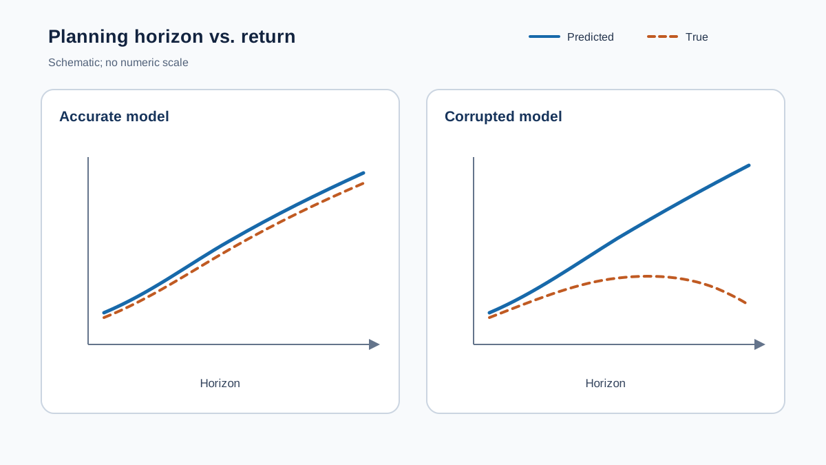
Now sweep H from 1 to 8 at two error levels and print the table.
for eps in (0.0, 0.3):
    print(f"\nepsilon = {eps}")
    print(f"{'H':>2} {'predicted':>10} {'true':>8}")
    for H in range(1, 9):
        m = make_model(eps, np.random.default_rng(42))
        pred, true = run_episode(m, H)
        print(f"{H:>2} {pred:>10.3f} {true:>8.3f}")
At epsilon = 0.0, predicted and true returns track each other closely, and longer horizons generally help — the planner sees further down a correct path. That is the case where the conventional advice holds.
At epsilon = 0.3, the two columns split. Predicted return keeps climbing with H because the planner is optimizing inside its own corrupted world. True return flattens, then falls. The planner is not confused. It is certain — and wrong. Each rollout step multiplies the model's error, so the value estimate drifts away from the state the agent will actually occupy.
Track action quality alongside the returns: at each H, does the selected action match the true-optimal action? You will typically see agreement stay high at short horizons and decay as H grows under error.
This is not a quirk of the toy. When a model is estimated from data, the planning horizon acts as a complexity control parameter — a shorter horizon defines a simpler policy class, which reduces overfitting to model error. The research result is that a shorter planning horizon can beat the true horizon precisely because it trades some foresight for less error accumulation. Your table is a miniature of that finding.
| Regime | Longer horizon | Shorter horizon |
|---|---|---|
| Accurate model | Usually helps | Leaves value on the table |
| Noisy model | Predicted return rises, true return falls | Often wins |
| Very noisy model | Every horizon looks equally bad | Still bad — fix the model |
Knowledge check
Check your understanding
Answer this question before you continue.
Failure Modes and Debugging Signals
When the experiment misbehaves, the symptom tells you which part is broken.
- Predicted return identical across all horizons. The error injection is not reaching the states the planner visits. Print the corruption table and check which states actually get redirected.
- True return flat or random. The execution loop is not using
TRUE, or the goal reward is unreachable from the start. VerifyTRUE[START]leads somewhere useful. - Planner always picks the same action. Tie-breaking or a single dominant path is hiding the horizon effect. Add a small random tie-break or a second start state.
epsilontoo high. The model becomes pure noise and every horizon looks equally bad. That teaches nothing. Start at0.1and step up.- Sanity check. Set
epsilon = 0and confirm the planner matches a brute-force optimal policy before trusting any other run. If it does not, the bug is in the planner, not the model.
Common mistake: Treating a rising predicted return as evidence the planner is improving. Under model error, predicted return is the least trustworthy number on the screen. The true return is the one that pays rent.
Knowledge check
Check your understanding
Answer this question before you continue.
Modify It: Replanning Frequency and Error Structure
One run is a data point. The interesting work is finding what flips the recommendation.
Change replanning frequency. Execute the full H-step plan before replanning, versus one step at a time. Replanning every step lets the agent correct drift immediately; committing to the whole plan exposes it to accumulated error. Compare decision quality across both.
Change error structure. Uniform random corruption is the easy case. A systematic bias — say, the model always overestimates progress toward the goal in one region — is closer to real learned models and often produces a sharper crossover.
Add a terminal value estimate. Instead of returning 0.0 at the horizon, plug in a rough value estimate. Under moderate error, this can rescue long horizons by giving the truncation something better than zero to stand on.
Record which modification moves the crossover point between short and long horizons. That crossover is the thing you actually care about.
What to Take Away
Horizon is not a free parameter you maximize. It is a trade between foresight and error accumulation, and the exchange rate depends entirely on how wrong your model is.
Three rules to carry forward:
- Measure predicted versus true outcome, not just predicted return. A planner can look better on paper and act worse in the world.
- When your model is estimated from limited data, test shorter horizons and frequent replanning before assuming longer is better. The complexity argument is real, and it has a measurable signature.
- Set the horizon by experiment, not by convention. The crossover point is empirical.
Your next step: replace the hand-written error injection with a model fit on a small sample of transitions. Sample a handful of real transitions, fit a simple tabular model, and rerun the same sweep. If the same crossover appears — predicted return rising while true return falls — you have reproduced the core failure of model-based planning on your own terms. That is the experiment worth running.
Knowledge check
Final check
Finish the article by checking the ideas you just learned.
References
Build a stronger RL mental model
Use structured resources to connect equations, algorithms, and observable agent behavior.


