
Deriving the Q-Learning Update: Targets, Learning Rates, and a Worked Example
You can copy the Q-learning update into code and watch it work. Then someone asks why the target uses the best next action when the agent just took a…

Key topics
You can copy the Q-learning update into code and watch it work. Then someone asks why the target uses the best next action when the agent just took a random one, and the formula turns back into a ritual.
Let's fix that. By the end of this article you will write the target from memory, explain why it ignores the action the agent actually took, and compute one update by hand.
This assumes you have already met Q-learning at the intuition level: that Q(s, a) estimates the return from taking action a in state s, and that the agent picks actions with an epsilon-greedy behavior policy. If that is still fuzzy, the concept-level treatment is the better starting point. Here we stay strictly in the tabular setting — finite states, finite actions, one update at a time, no neural networks.
The Setting and the Symbols
Before the derivation, pin down what each symbol measures and what changes when it grows or shrinks.
| Symbol | Meaning | What it controls |
|---|---|---|
| s | current state | where the agent is right now |
| a | action taken in s | the decision being evaluated |
| r | reward observed after the step | the immediate signal |
| s′ | next state | where the agent landed |
| γ (gamma) | discount factor, between 0 and 1 | how much future value counts today |
| α (alpha) | learning rate, between 0 and 1 | how far one sample moves the estimate |
| Q(s, a) | table entry for this state-action pair | the current estimate of return |
The assumptions matter as much as the symbols. The update is valid when states and actions are discrete and enumerable, the table can physically hold every pair, and a reward arrives after each step. It also assumes the Markov property: the current state and action contain everything needed to predict what comes next. In plain terms, if two situations look identical to the agent but lead to different futures, the state is hiding information and the table cannot learn reliably from it. Step outside those conditions — continuous states, millions of states, or a state space you cannot enumerate — and the table stops being a table. That is the boundary where function approximation takes over, and it is a later topic.
Knowledge check
Check your understanding
Answer this question before you continue.
From Return to Target: Why the Update Looks Like This
Start with the definition, not the formula. The action value is the expected discounted return after taking a in s:
That infinite sum is useless as written. So decompose it one step at a time. The first reward is immediate; everything after it is just the return from the next state, discounted once:
This is the Bellman idea in one line: value now equals reward now plus discounted value later. The expectation averages over whatever action the policy would take next. But the true next-state value is unknown — that is the whole problem. So we substitute our current table estimate for it. That substitution is the bootstrap step: we learn from an estimate instead of waiting for the full return.
Now the part that trips people up. That expectation describes the return under a specific policy — the one choosing a′. Q-learning does not want the value of that policy. It wants the value of acting optimally from the next state onward. So instead of averaging over the next action, it takes the max over the table:
This is not algebraic substitution inside the previous equation. It is a different target: the Bellman optimality backup, which asks if I acted optimally from the next state onward, what would this transition be worth? The max selects the best estimated next action, and that greedy choice is what makes Q-learning learn the optimal policy rather than the policy it happens to be following.
One more shift matters for the tabular update. The equations above describe expected quantities — averages over many possible transitions. A single update does not have the average. It has one sampled transition: the reward r you actually received and the next state s′ you actually landed in. The table supplies the bootstrap estimate for that s′. So the target you compute on any given step is a sampled, one-step version of the optimality backup:
The gap between this target and the current estimate is the temporal-difference error:
Finally, move the estimate a fraction α toward the target:
Written as a weighted average, the same update reads:
Old estimate on one side, new evidence on the other, blended by α. That is the entire Q-learning update rule derivation — no ritual left, just a one-step Bellman decomposition, a bootstrap, and a greedy max.
Knowledge check
Check your understanding
Answer this question before you continue.
What the Learning Rate and Discount Factor Actually Do
α controls how far one sample moves the estimate. Small α averages over many noisy samples; large α chases the latest one. Neither is correct in isolation — the useful range depends on reward scale and how often each state-action pair gets visited.
γ controls how much a future estimate counts today. It sets the horizon. With γ near 1, the agent cares about distant rewards, and the target inherits the noise of the next-state estimate. With γ near 0, it behaves almost greedily toward immediate reward. A discount below 1 also keeps values finite in continuing tasks, where the return would otherwise sum forever.
Here is the interaction that trips people up: γ near 1 plus a noisy table means the target is mostly borrowed value. You are not learning from the reward; you are learning from your own guess about the future. That is fine when the guess improves over time, and dangerous when it does not.
Common mistake: Treating α and γ as universal constants. They are not magic numbers. Their useful range depends on reward scale, visit frequency, and how noisy your estimates are.
Knowledge check
Check your understanding
Answer this question before you continue.
A Worked Update, Number by Number
Take a three-state corridor: S0 → S1 → S2, with actions Left and Right. Reaching S2 from S1 gives reward +1; every other step gives 0. Use α = 0.5 and γ = 0.9.
Before the update, the relevant slice of the Q-table:
| State | Left | Right |
|---|---|---|
| S0 | 0.0 | 0.0 |
| S1 | 0.0 | 0.0 |
| S2 | 0.0 | 0.0 |
The agent is in S1, takes Right (an exploratory pick), observes r = +1, and lands in S2.
Step 1 — greedy next-state value. Read the max from the S2 row: max(0.0, 0.0) = 0.0.
Step 2 — target. r + γ · max = 1 + 0.9 · 0.0 = 1.0.
Step 3 — TD error. δ = 1.0 − Q(S1, Right) = 1.0 − 0.0 = 1.0.
Step 4 — apply α. Q(S1, Right) ← 0.0 + 0.5 · 1.0 = 0.5.
After the update, exactly one cell changed:
| State | Left | Right |
|---|---|---|
| S0 | 0.0 | 0.0 |
| S1 | 0.0 | 0.5 |
| S2 | 0.0 | 0.0 |
Now repeat the same transition. The target is still 1 + 0.9 · 0.0 = 1.0, but the estimate is now 0.5, so δ = 0.5 and Q(S1, Right) ← 0.5 + 0.5 · 0.5 = 0.75. Run it again and you get 0.875. Each pass halves the gap to the target — the estimate is converging, not jumping.
Knowledge check
Check your understanding
Answer this question before you continue.
Why the Target Ignores the Action the Agent Took
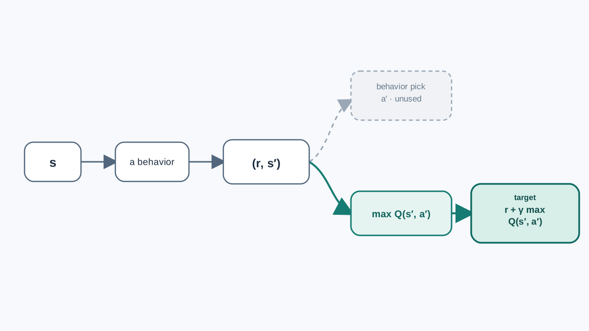
Look back at the update. It used s, a, r, and s′. It never asked what action the agent chose in s′. That omission is the whole off-policy story.
Two policies are in play. The behavior policy picks actions during data collection — here, epsilon-greedy, so it sometimes picks randomly. The greedy policy is implied by the max in the target: it always assumes the best next action. Q-learning learns the value of the greedy policy while behaving according to the exploratory one. That is what "off-policy" means mathematically: the target is computed under a different policy than the one generating the data.
The practical consequence is liberating. You can explore aggressively — even take mostly random actions — without corrupting the value you are learning. The target corrects for your wandering by asking what the best action would have been.
Warning: A max over noisy estimates can look better than reality, because you are selecting the largest of several uncertain numbers. That overestimation bias is a real failure mode and deserves its own treatment.
This is also exactly where Q-learning parts ways with its on-policy cousin, which uses the next action actually taken instead of the max. That comparison is covered elsewhere; here, just note the fork in the road.
When This Update Is the Right Tool
Use the tabular update when states and actions are discrete, enumerable, and visited often enough that each cell gets updated many times. Do not expect it to scale to large or continuous state spaces — a table you cannot fill is not a table.
The tradeoff is data efficiency: each update uses a single transition, so learning depends on repeated coverage. Sparse visits mean slow learning, and cells you never touch never improve.
Here is your next move. Implement the update in a few lines, run the tiny corridor, and print the Q-table after every episode. Watch the value at S1 climb, then watch it propagate backward into S0 one cell at a time as the reward reaches further back through the chain. That backward creep is credit assignment made visible — and it is the mechanism the formula was always describing.
Knowledge check
Final check
Finish the article by checking the ideas you just learned.
References
Build a stronger RL mental model
Use structured resources to connect equations, algorithms, and observable agent behavior.


